HPC Notes

DNDSR designs

Array data structure

Array<>

The basic Array<T,...> data container is a data container designed for MPI-based distributed parallelism. Element type T has to be trivially-copyable.

1
2
3
4
5
6
7
8
9
template <class T, rowsize _row_size = 1, rowsize _row_max = _row_size, rowsize _align = NoAlign>
class Array : public ArrayLayout<T, _row_size, _row_max, _align>
{
    ...
    // holds data (and indexing)
    // methods for indexing
    // methods for serialization
    // methods for device
};

	_row_size>=0	_row_size==DynamicSize	_row_size==NonUniformSize
_row_max>=0	TABLE_StaticFixed	TABLE_Fixed	TABLE_StaticMax
_row_max==DynamicSize	TABLE_StaticFixed_row_max ignored	TABLE_Fixed_row_max ignored	TABLE_Max
_row_max==NonUniformSize	TABLE_StaticFixed_row_max ignored	TABLE_Fixed_row_max ignored	CSR

Underlying data layout: 1-D indexing / 2-D indexing.

For fix-sized 2-D tables, it is basically a row-major matrix with the first index potentially globally aware. For variable-sized 2-D tables, it is a CSR-indexed variable array.

ParArray<> and ArrayTransformer<>

Parallel communication: ParArray<...> and ArrayTransformer<...>.

ParArray is Array with global indexing info. Generally use a globally (inside the MPI communicator) rank-based contiguous indexing. Operations on ParArray should be collaborative (inside MPI comm).

1
2
3
4
5
6
7
template <class T, rowsize _row_size = 1, rowsize _row_max = _row_size, rowsize _align = NoAlign>
class ParArray : public Array<T, _row_size, _row_max, _align>
{
    ...
    // holds rank-global indexing data
    // global indexing methods
};

ArrayTransformer<...> relates two ParArray<...> together by defining an all-to-all style arbitrary index mapping.

 1
 2
 3
 4
 5
 6
 7
 8
 9
10
template <class T, rowsize _row_size = 1, rowsize _row_max = _row_size, rowsize _align = NoAlign>
class ArrayTransformer
{
    ...
    // reference father & son arrays
    // ghost mapping data (father->son index mapping)
    // MPI data types
    // MPI requests
    // pull and push methods
};

In PDE solvers, most used critical for ghost mesh/point/cell data, so the mapping is called ghost mapping.

Conceptually:

1
ArrSon[IndexSon] = ArrFather[IndexFather]

We define that IndexFather can be scattered in each rank (section) or even overlapping, and IndexSon must be like 0:N. Therefore, transforming from father to son (or main to ghost) is unique, but not so backwards.

We name father->son parallel data transferring pull, and push when reversed.

General communication procedures:

 1
 2
 3
 4
 5
 6
 7
 8
 9
10
11
12
13
ParArray<...> arrFather(...);
ParArray<...> arrSon(...);
...
// initialize Father's data
ArrayTransformer<...> arrTrans(...);
...
// set arrTrans to refer to arrFather and arrSon
arrFather.createGlobalMapping();
...
// prepare pullingIndex
arrTrans.createGhostMapping(pullingIndex); 
arrTrans.createMPITypes();// automatically reshape arrSon to match arrFather
arrTrans.pullOnce(); // or InitPersistentPull();

For persistent data transfers:

1
2
3
4
5
6
7
arrTrans.InitPersistentPull();
// each iteration
{
    arrTrans.StartPersistentPull();
    ...
    arrTrans.WaitPersistentPull();
}

To ease the use of underlying data, we have ArrayEigenMatrix<...> for AoS style floating point DOF storage, and ArrayAdjacency<...> for integer index storage. They inherit from ParArray<>.

ArrayPair<>

Sometimes a pair of father and son are always bound together to form a main vs. ghost pair.

To ease the complexity of data indexing in the ghost region, ArrayTransformer’s ghost indexing can be stored as a local version of adjacency table. We define that the local index of ghost is appended to the main part, so that a local adjacency table can be logically valid and compact. This indexing and pairing is realized by the wrapper ArrayPair<>.

1
2
3
4
5
6
7
8
template <class TArray = ParArray<real, 1>>
struct ArrayPair
{
    // reference father and son arrays
    // hold the ArrayTransformer
    // indexing methods (with appending range)
    // ...
};

DeviceView

The hierarchy of Array data containers can generate a trivially-copyable device view objects that only hold pointers and sizes and have data-accessors methods that never mutate the array shape.

The device views may hold device pointers, which make them perfectly usable on CUDA devices.

Some shared data, like CSR indexes can be forced into a raw-pointer to reduce overhead (on CPU).

Device views should always be generated and used in a local procedure during which the array shapes are never mutated.

Asynchronous procedures

A direct design:

 1
 2
 3
 4
 5
 6
 7
 8
 9
10
11
ArrayPair a, b;
... // previous computing
a.trans.waitPersistentPull();
computeA(a); // reads a, writes a
a.trans.startPersistentPull();

... // some independent computing

a.trans.waitPersistentPull();
computeA2B(a, b); // reads a, writes b
b.trans.startPersistentPull();

A more sophisticated design:

1
2
3
4
5
6
7
8
ArrayPair a, b;
... // previous computing
a.trans.startPersistentPull();

computeA2BMain(a, b); // reads a's main part, writes b
a.trans.waitPersistentPull();
computeA2BGhost(a, b); // reads a's main+ghost part, writes b
b.trans.startPersistentPull();

A more robust interface: TASK BASED

Task based scheduling

1. Core abstraction: tasks, data regions, and access modes

1.1 Data objects with regions

Instead of thinking in terms of arrays + ghost exchange, define logical data objects with regions:

1
2
3
4
5
Data a("a"), b("b");

// Regions (can be arbitrary subsets)
Region a_main  = a.region("main");
Region a_ghost = a.region("ghost");

The runtime understands that:

a_main is local
a_ghost requires MPI communication

1.2 Tasks with access descriptors

Each task declares what data it accesses and how:

 1
 2
 3
 4
 5
 6
 7
 8
 9
10
11
12
13
task ComputeA {
    read_write(a_main);
}

task ComputeA2BMain {
    read(a_main);
    write(b_main);
}

task ComputeA2BGhost {
    read(a_main, a_ghost);
    write(b_main);
}

This is the only information the scheduler needs.

2. Communication becomes implicit tasks

MPI communication is not special — it is just another task:

1
2
3
4
task PullGhost {
    read(a_remote);
    write(a_ghost);
}

The runtime inserts this automatically when:

A task reads a region that is not locally available

3. DAG construction (formal model)

Each iteration builds a directed acyclic graph (DAG):

Nodes

Compute tasks
Communication tasks (MPI Isend/Irecv)
Optional memory transfer tasks (H2D, D2H, disk I/O)

Edges

T1 → T2 if T2 needs data produced by T1

4. Scheduler semantics (key rules)

A runtime loop looks like this:

1
2
3
4
5
6
7
8
while (!all_tasks_done) {
    for task in tasks {
        if (resources_available(task)) {
            launch(task);
        }
    }
    progress_communication();  // MPI_Test, MPI_Waitsome
}

Task readiness condition

A task is ready if:

All its input regions are available
No conflicting write is in flight

5. Pseudo-code: user-facing API

 1
 2
 3
 4
 5
 6
 7
 8
 9
10
11
12
13
14
Graph g;

g.add_task("ComputeA")
  .reads_writes(a_main);

g.add_task("ComputeA2BMain")
  .reads(a_main)
  .writes(b_main);

g.add_task("ComputeA2BGhost")
  .reads(a_main, a_ghost)
  .writes(b_main);

execute(g);

6. Runtime-side pseudo-code

6.1 Dependency resolution (for distributed memory)

As non-local dependency should automatically create some comm tasks:

1
2
3
4
5
for task in graph:
    for region in task.reads:
        if (!region.is_available()):
            insert_comm_task(region)
            add_edge(comm_task, task)

6.2 Communication task

1
2
3
4
task CommTask(region) {
    MPI_Irecv(region.buffer);
    MPI_Isend(...);
}

Completion of CommTask marks region as available.

7. Exploiting task parallelism within a rank

Once everything is tasks, intra-node parallelism is automatic:

1
2
3
4
5
6
7
#pragma omp parallel
{
    while (scheduler.has_work()) {
        Task t = scheduler.get_ready_task();
        t.run();
    }
}

Python interface

DNDSR has a Python interface that allow orchestration of the computing via Python.

Core concept: Array, ParArray, ArrayTransformer, ArrayPair are exported to Python via pybind11.

In python: provide (CPU-side) data accessors (mostly for testing or initializations).

Export mesh and solver interface, including mesh data (adjacency and geometry), solver data (FV’s geometric data), relevant methods, computing methods (kernels).

To collaborate with other libraries:

numpy is natural, via buffer protocol
mpi4py is compiled in the same MPI env.
cupy is compiled in the same CUDA env (runtime linking?)

DNDSR CUDA kernels

DNDSR provide CUDA capabilities.

Each Array actually holds data via a host_device_vector<T> object.

host_device_vector is like std::vector or thrust::device_vector but provides a unified interface.

It uses an underlying DeviceStorageBase for byte storage that may be implemented on various devices.

 1
 2
 3
 4
 5
 6
 7
 8
 9
10
11
class DeviceStorageBase
{
public:
    virtual uint8_t *raw_ptr() = 0;
    virtual void copy_host_to_device(uint8_t *host_ptr, size_t n_bytes) = 0;
    virtual void copy_device_to_host(uint8_t *host_ptr, size_t n_bytes) = 0;
    virtual void copy_to_device(uint8_t *device_ptr_dst, size_t n_bytes) = 0;
    [[nodiscard]] virtual size_t bytes() const = 0;
    [[nodiscard]] virtual DeviceBackend backend() const = 0;
    virtual ~DeviceStorageBase();
};

Array objects then can do to_device… and to_host to initiate H2D / D2H data transfer.

Currently no async memcpy interface provided.

To pass device-stored Array objects (and derived/combined ones) to CUDA kernels, they provide device view generators that generate trivially copyable XXDeviceView objects.

To reduce the size of Array device views, currently std::conditional_t<...> is used for its data fields. If some pointer/size is not needed, the data field is set to Empty type. Due to C++ standard, a simple empty struct still takes 1 byte as member data, could use [[no_unique_address]] if upgrade to C++ 20.

The device view objects can be passed directly as parameters of __global__ functions.

However, one limitation is that some objects composed of a large amount of ArrayXXXs can generate huge device view objects. For example, EulerP::EvaluatorDeviceView<B>, which holds an FV view and a mesh view, takes up 3496 bytes because they hold/reference dozens of ArrayPairs.

In such cases, nvcc might complain about the parameter size being too large. A safe way is to store the view into global memory before calling the kernel and passing the global pointer.

For huge-view storage, as they do not change (during kernel), and are basically broadcasted, using constant memory should be better. However, managing the total constant memory size per CUDA context need more infrastructure.

Currently, for CUDA-resided Arrays, ArrayTransformer is only able to handle MPI communication via a CUDA-aware MPI.

EulerP CUDA implementation

See the test here: EulerP CUDA tests

Currently, for 2nd-order finite-volume kernels, we use simple one-thread-per-point parallelism.

Each thread writes to one point, write buffer pattern is known.

Each thread reads several points, read buffer pattern is decided by the mesh adjacency (graph).

Computing density is quite low, almost 1 ~ 3 op / 8 bytes ! Read pattern is unstable, not easy to reuse read buffer. Use graph reordering to improve locality for L2-cache friendliness ?.

What we can do first?

Write coalescing optimization

The DOFs of DNDSR are packed as AoS style: $N\times 5$ row-major matrix, where threads are mapped onto $N$’s dimension for computing.

For gradients, this becomes $N\times 15$.

If extend to higher order methods, the row size could be much larger.

Some auxiliary arrays (and extended scalar DOFs) are stored as SoA style, but the primary N-S Dofs are packed together as they are always used as a whole.

Moreover, as the solver is designed to be an N-S coupled solver, block-sparse matrix must accept a SOA-style array as DOF.

Therefore, no cheap coalescing, need manual shuffling. A rather generic wrapped __device__ function for this optimization:

 1
 2
 3
 4
 5
 6
 7
 8
 9
10
11
12
13
14
15
16
17
18
19
20
21
22
23
24
25
26
27
28
29
30
31
32
33
34
35
36
37
38
39
40
41
42
43
44
45
template <int local_stride_fixed, int max_tid_fixed,
            class TFLocalAccessor, class TFGlobalAccessor,
            int bufferSize_idx, int bufferSize_val>
DNDS_FORCEINLINE DNDS_DEVICE void CUDA_Local2GlobalAssign(
    TFLocalAccessor &&FLocalAccessor,
    TFGlobalAccessor &&FGLobalAccessor,
    CUDA::SharedBuffer<index, bufferSize_idx> &shared_buf_idx,
    CUDA::SharedBuffer<real, bufferSize_val> &shared_buf_val,
    index iPnt, index iPntMax)
{
#    ifndef __CUDA_ARCH__
    static_assert(local_stride_fixed > 0 && local_stride_fixed < 0);
#    endif
    static_assert(local_stride_fixed > 0);
    static_assert(max_tid_fixed > 0);
    static_assert(bufferSize_idx >= max_tid_fixed);
    // TODO: support dynamic sized?

    constexpr int local_stride = local_stride_fixed;
    constexpr int local_stride_buf = (local_stride / 2) * 2 + 1;
    static_assert(bufferSize_val >= local_stride_buf * max_tid_fixed);

    real *buf_data = shared_buf_val.buffer;
    index *iPntThread = shared_buf_idx.buffer;

    int tid = CUDA::tid_x();
    int bDim = CUDA::bDim_x();
    DNDS_HD_assert(tid < max_tid_fixed && tid >= 0);
    iPntThread[tid] = iPnt; //! can out of bounds
    for (int i = 0; i < local_stride; i++)
        buf_data[tid * local_stride_buf + i] = FLocalAccessor(i);

    CUDA::sync_threads();
    for (int i = 0; i < local_stride; i++)
    {
        int iComp = (i * bDim + tid);
        int iPntInBlock = iComp / local_stride;
        int iCompSub = iComp % local_stride;
        int iCompBuf = (local_stride == local_stride_buf) ? iComp : (iPntInBlock * local_stride_buf + iCompSub);
        // int iComp = (i * bDim + tid) % local_stride;
        index iPntC = iPntThread[iPntInBlock];
        if (iPntC < iPntMax)
            FGLobalAccessor(iPntC, iCompSub) = buf_data[iCompBuf];
    }
}

This is thread-block level synchronized call, do not diverge on the call.

Template instantiation divergence could cause serious problems, the safest pattern is to call only once.

Effect: 3.2x speed boost, 2.8x power efficiency boost.

CUDA

Sort

Bitonic

Purely in-block sort: bitonic sort

 1
 2
 3
 4
 5
 6
 7
 8
 9
10
11
12
13
14
15
16
17
18
19
20
21
22
23
24
25
26
27
28
29
30
31
32
33
34
35
36
37
38
39
40
41
42
43
44
45
46
47
48
49
50
51
52
53
54
55
56
57
template <typename T>
__device__ inline bool less_than(T a, T b)
{
    return a < b;
}

template <typename T>
__device__ inline T biggest()
{
    if constexpr (std::is_same_v<T, float>)
        return FLT_MAX;
    else
        static_assert(std::is_same_v<T, float>, "type is not supported");

    return 0;
}

template <typename T>
__global__ void bitonic_sort_1d(T *data, int N)
{
    extern __shared__ T sdata[];
    int tid = threadIdx.x;
    int bdim = blockDim.x;

    if (tid < N)
        sdata[tid] = data[tid];
    else
        sdata[tid] = biggest<T>();
    __syncthreads();

    // Bitonic sort
    for (int k = 2; k <= bdim; k <<= 1) // merge length
    {
        for (int j = k >> 1; j > 0; j >>= 1) // compare stride
        {
            int ixj = tid ^ j; // compare partner

            if (ixj > tid)
            {
                bool ascending = ((tid & k) == 0);
                T a = sdata[tid];
                T b = sdata[ixj];

                if ((ascending && less_than(b, a)) ||
                    (!ascending && less_than(a, b))) // then swap
                {
                    sdata[tid] = b;
                    sdata[ixj] = a;
                }
            }
            __syncthreads();
        }
    }

    if (tid < N)
        data[tid] = sdata[tid];
}

Radix

For bit 0, get bucket counts: total_zeros and predicate is_zero[i]
scan predicate: prefix sum (exclusive) prefix_zero[i]
scatter:

 1
 2
 3
 4
 5
 6
 7
 8
 9
10
11
12
13
14
15
16
17
18
19
__global__ void scatter(
    const uint32_t* in,
    uint32_t* out,
    const int* is_zero,
    const int* prefix_zero,
    int total_zeros,
    int N
) {
    int i = blockIdx.x * blockDim.x + threadIdx.x;
    if (i < N) {
        if (is_zero[i]) {
            int pos = prefix_zero[i];
            out[pos] = in[i];
        } else {
            int pos = total_zeros + (i - prefix_zero[i]);
            out[pos] = in[i];
        }
    }
}

Do bit 1 sorting in segments out[0:total_zeros], out[total_zeros:]
…

Optimizations

Using b bits together. b=4, 16 buckets.

Each element belongs to 1 bucket.

Block-wise histogram: hist[iBlock][iBucket]

Global block-hist: hist_g[iBucket] -> prefix sum of the 16 sized array: bucket_start[iBucket]

Prefix sum on block-hist: hist_ps[iBlock][iBucket]

Then element-wise prefix-sum per-block (in-block scanning) pre_num[iBucket][tid] (only locally used so no actual global mem).

The new index: pre_num[iBucket][tid] + hist_ps[iBlock][iBucket] + bucket_start[iBucket]

Block scanning

 1
 2
 3
 4
 5
 6
 7
 8
 9
10
11
12
13
14
15
16
17
18
19
20
21
22
23
24
25
26
27
28
29
30
31
32
33
34
35
36
37
__shared__ int s[];

int tid = threadIdx.x;

// load
s[tid] = input[gid];
__syncthreads();

// up-sweep
for (int offset = 1; offset < blockDim.x; offset <<= 1) {
    int idx = (tid + 1) * offset * 2 - 1;
    if (idx < blockDim.x)
        s[idx] += s[idx - offset];
    __syncthreads();
}

// store block sum
if (tid == blockDim.x - 1)
    block_sum[blockIdx.x] = s[tid];

// down-sweep
if (tid == 0)
    s[blockDim.x - 1] = 0;
__syncthreads();

for (int offset = blockDim.x >> 1; offset > 0; offset >>= 1) {
    int idx = (tid + 1) * offset * 2 - 1;
    if (idx < blockDim.x) {
        int t = s[idx - offset];
        s[idx - offset] = s[idx];
        s[idx] += t;
    }
    __syncthreads();
}

// write output
output[gid] = s[tid];

Working example

  1
  2
  3
  4
  5
  6
  7
  8
  9
 10
 11
 12
 13
 14
 15
 16
 17
 18
 19
 20
 21
 22
 23
 24
 25
 26
 27
 28
 29
 30
 31
 32
 33
 34
 35
 36
 37
 38
 39
 40
 41
 42
 43
 44
 45
 46
 47
 48
 49
 50
 51
 52
 53
 54
 55
 56
 57
 58
 59
 60
 61
 62
 63
 64
 65
 66
 67
 68
 69
 70
 71
 72
 73
 74
 75
 76
 77
 78
 79
 80
 81
 82
 83
 84
 85
 86
 87
 88
 89
 90
 91
 92
 93
 94
 95
 96
 97
 98
 99
100
101
102
103
104
105
106
107
108
109
110
111
112
113
114
115
116
117
118
119
120
121
122
123
124
125
126
127
128
129
130
131
132
133
134
135
136
137
138
139
140
141
142
143
144
145
146
147
148
149
150
151
152
153
154
155
156
157
158
159
160
161
162
163
164
165
166
167
168
169
170
171
172
173
174
175
176
177
178
179
180
181
182
183
184
185
186
187
188
189
190
191
192
193
194
195
196
197
198
199
200
201
202
203
204
205
206
207
208
209
210
211
212
213
214
215
216
217
218
219
220
221
222
223
224
225
226
227
228
229
230
231
232
233
234
235
236
237
238
239
240
241
242
243
244
245
246
247
248
249
250
251
252
253
254
255
256
257
258
259
260
261
262
263
264
265
266
267
268
269
270
271
272
273
274
275
276
277
278
279
280
281
282
283
284
285
286
287
288
289
290
291
292
293
294
295
296
297
298
299
300
301
302
303
304
305
306
307
308
309
310
311
312
313
314
315
316
317
318
319
320
321
322
323
324
325
326
327
328
329
330
331
332
333
334
335
336
337
338
339
340
341
342
343
344
345
346
347
348
349
350
351
352
353
354
355
356
357
358
359
360
361
362
363
364
365
366
367
368
369
370
371
372
373
374
375
376
377
378
379
380
381
382
383
384
385
386
387
388
389
390
391
392
393
394
395
396
397
398
399
400
401
402
403
404
405
406
407
408
409
410
411
412
413
414
415
416
417
418
419
420
421
422
423
#pragma once

#include <cuda_runtime.h>
#include <cstdint>
#include <cassert>
#include <iostream>
#include <vector>

#define CUDA_CHECK_LAST()                                         \
    do                                                            \
    {                                                             \
        cudaError_t err = cudaGetLastError();                     \
        if (err != cudaSuccess)                                   \
        {                                                         \
            fprintf(stderr,                                       \
                    "CUDA kernel launch error %s:%d: %s\n",       \
                    __FILE__, __LINE__, cudaGetErrorString(err)); \
            abort();                                              \
        }                                                         \
    } while (0)

template <typename T>
void debugPrintDeviceArray(const T *d_ptr, size_t count,
                           const char *label = nullptr,
                           size_t max_print = 256)
{
    if (label)
    {
        std::cout << label << " ";
    }
    std::cout << "(count=" << count << "):\n";

    if (count == 0 || d_ptr == nullptr)
    {
        std::cout << "  <empty>\n";
        return;
    }

    size_t n = std::min(count, max_print);

    std::vector<T> h_buf(n);

    cudaError_t err = cudaMemcpy(
        h_buf.data(), d_ptr, n * sizeof(T), cudaMemcpyDeviceToHost);

    if (err != cudaSuccess)
    {
        std::cerr << "cudaMemcpy failed: "
                  << cudaGetErrorString(err) << "\n";
        return;
    }

    for (size_t i = 0; i < n; ++i)
    {
        std::cout << h_buf[i] << ", ";
    }

    if (n < count)
    {
        std::cout << "...";
    }
    std::cout << "\n";
}

constexpr int n_bit = 4;
constexpr int n_bucket = 1 << n_bit;
constexpr unsigned int partial_mask = (0xFFFFFFFFu << n_bit) ^ 0xFFFFFFFFu;

constexpr int warp_size = 32;
constexpr int warps_per_block = 32;
constexpr int tpb = warp_size * warps_per_block;
constexpr uint32_t warp_mask = 1ull << warps_per_block - 1;

constexpr int cdiv(int a, int b) { return (a + b - 1) / b; }

#ifdef NDEBUG
#undef NDEBUG
#endif

__device__ __forceinline__ int warp_reduction(int val, uint32_t mask = 0xFFFFFFFFu)
{
    for (int offset = warp_size / 2; offset > 0; offset >>= 1)
    {
        val += __shfl_down_sync(mask, val, offset);
    }
    return val;
}

__global__ void get_block_counting_histogram(const unsigned int *input, int *block_histogram /*n_bucket * n_blks*/,
                                             int *global_histogram, int N, int n_blks, int iMask)
{
    const int tid_g = threadIdx.x + blockDim.x * blockIdx.x;
    const int tid = threadIdx.x;
    const int lane = tid % warp_size;
    const int wid = tid / warp_size;

    const unsigned int mask = partial_mask << (n_bit * iMask);

    unsigned int input_c = 0xFFFFFFFFu;
    if (tid_g < N)
        input_c = input[tid_g];
    unsigned int partial_key = (input_c & mask) >> (n_bit * iMask);

    __shared__ int warp_results[n_bucket][warp_size];
    static_assert(warps_per_block <= warp_size);

    for (int i = 0; i < n_bucket; i++)
    {
        int sum = warp_reduction(partial_key == i ? 1 : 0);
        if (lane == 0)
            warp_results[i][wid] = sum;
    }
    __syncthreads();

    if (wid == 0)
    {
        for (int i = 0; i < n_bucket; i++)
        {
            int sum = warp_reduction(warp_results[i][lane], warp_mask);
            if (lane == 0)
            {
                block_histogram[i * n_blks + blockIdx.x] = sum;
                atomicAdd(global_histogram + i, sum);
            }
        }
    }
}

__device__ __forceinline__ int warpInclusiveScan(int lane, int val, unsigned mask = 0xffffffff)
{

    for (int offset = 1; offset < warp_size; offset <<= 1)
    {
        int n = __shfl_up_sync(mask, val, offset);
        if (lane >= offset)
            val += n;
    }
    return val;
}

__global__ void global_histogram_to_prefix_sum(int *histo)
{
    const int tid_g = threadIdx.x + blockDim.x * blockIdx.x;
    const int tid = threadIdx.x;
    const int lane = tid % warp_size;
    const int wid = tid / warp_size;
    
    static_assert(n_bucket <= tpb);

    __shared__ int warp_sums[1][warp_size];
    int results[1];
    
    int val = 0;
    if (tid_g < n_bucket)
        val = histo[tid_g];
    results[0] = warpInclusiveScan(lane, val);
    if (lane == warp_size - 1)
        warp_sums[0][wid] = results[0];
    results[0] -= val; // becomes exclusive scan result
    
    __syncthreads();
    if (wid == 0)
    {

        const int warp_sum = warp_sums[0][lane];
        const int warp_sum_scan = warpInclusiveScan(lane, warp_sum, warp_mask) - warp_sum;
        warp_sums[0][lane] = warp_sum_scan;
        // becomes exclusive scan sum
    }
    __syncthreads();


    results[0] += warp_sums[0][wid]; // block-wise prefix sum exclusive
    if (tid_g < n_bucket)
        histo[ tid_g] = results[0];
    
}

__global__ void block_histogram_to_partial_prefix_sum(
    const int *histogram, int *partial_prefix_sum, int *block_sum, int N)
{
    const int tid_g = threadIdx.x + blockDim.x * blockIdx.x;
    const int tid = threadIdx.x;
    const int lane = tid % warp_size;
    const int wid = tid / warp_size;

    __shared__ int warp_sums[n_bucket][warp_size];

    int results[n_bucket];
    for (int i = 0; i < n_bucket; i++)
    {
        int val = 0;
        if (tid_g < N)
            val = histogram[i * N + tid_g];
        results[i] = warpInclusiveScan(lane, val);
        if (lane == warp_size - 1)
            warp_sums[i][wid] = results[i];
        results[i] -= val; // becomes exclusive scan result
    }

    __syncthreads();

    if (wid == 0)
    {
        for (int i = 0; i < n_bucket; i++)
        {
            const int warp_sum = warp_sums[i][lane];
            const int warp_sum_scan = warpInclusiveScan(lane, warp_sum, warp_mask) - warp_sum;
            warp_sums[i][lane] = warp_sum_scan;
            // becomes exclusive scan sum
            if (lane == warp_size - 1) // last one
            {
                block_sum[i * gridDim.x + blockIdx.x] = warp_sum_scan + warp_sum;
            }
        }
    }

    __syncthreads();

    for (int i = 0; i < n_bucket; i++)
    {
        results[i] += warp_sums[i][wid]; // block-wise prefix sum exclusive
        if (tid_g < N)
            partial_prefix_sum[i * N + tid_g] = results[i];
    }
}

__global__ void partial_prefix_sum_to_global_prefix_sum(
    int *partial_prefix_sum, const int *block_sum_prefix_sum, int N)
{
    const int tid_g = threadIdx.x + blockDim.x * blockIdx.x;
    // const int tid = threadIdx.x;
    // const int lane = tid % warp_size;
    // const int wid = tid / warp_size;

    for (int i = 0; i < n_bucket; i++)
    {
        if (tid_g < N)
            partial_prefix_sum[i * N + tid_g] += block_sum_prefix_sum[i * gridDim.x + blockIdx.x];
    }
}

__global__ void scatter(const unsigned int *input, unsigned int *output,
                        const int *block_histogram_prefix_sum, const int *global_histogram_ibucket_prefix_sum,
                        int N, int n_blks, int iMask)
{
    const int tid_g = threadIdx.x + blockDim.x * blockIdx.x;
    const int tid = threadIdx.x;
    const int lane = tid % warp_size;
    const int wid = tid / warp_size;

    const unsigned int mask = partial_mask << (n_bit * iMask);

    unsigned int input_c = 0xFFFFFFFFu;
    if (tid_g < N)
        input_c = input[tid_g];
    unsigned int partial_key = (input_c & mask) >> (n_bit * iMask);

    __shared__ int warp_sums[n_bucket][warp_size];

    int results[n_bucket];
    for (int i = 0; i < n_bucket; i++)
    {
        int val = partial_key == i ? 1 : 0;
        results[i] = warpInclusiveScan(lane, val);
        if (lane == warp_size - 1)
            warp_sums[i][wid] = results[i];
        results[i] -= val; // becomes exclusive scan result
    }
    __syncthreads();
    if (wid == 0)
    {
        for (int i = 0; i < n_bucket; i++)
        {
            const int warp_sum = warp_sums[i][lane];
            const int warp_sum_scan = warpInclusiveScan(lane, warp_sum, warp_mask) - warp_sum;
            warp_sums[i][lane] = warp_sum_scan;
            // becomes exclusive scan sum
        }
    }

    __syncthreads();

    int idx_new = -1;
    for (int i = 0; i < n_bucket; i++)
    {
        results[i] += warp_sums[i][wid];                                   // block-wise prefix sum exclusive
        results[i] += block_histogram_prefix_sum[i * n_blks + blockIdx.x]; // global prefix sum of ith bucket
        results[i] += global_histogram_ibucket_prefix_sum[i];              // in global index
        if (i == partial_key)
        {
            idx_new = results[i];
        }
    }
    if (tid_g < N)
    {
        // printf("!! %d\n", idx_new);
        output[idx_new] = input[tid_g];
    }
}

__host__ void sort_partial(const unsigned int *input, unsigned int *output, int N, int iMask,
                           int *buf, int *buf_end)
{
    // std::cout << iMask << std::endl;
    // printf("%x\n", partial_mask << (n_bit * iMask));
    int n_blocks = cdiv(N, tpb);

    int N_histo = n_bucket * n_blocks;
    int *global_histo = buf;
    buf += n_bucket;
    assert(buf <= buf_end);
    int *block_histo = buf;
    buf += N_histo;
    assert(buf <= buf_end);

    cudaMemset(global_histo, 0, sizeof(int) * n_bucket);
    get_block_counting_histogram<<<n_blocks, tpb>>>(input, block_histo,
                                                    global_histo, N, n_blocks, iMask);
    // debugPrintDeviceArray(input, N, "input");
    // debugPrintDeviceArray(block_histo, N_histo, "block_histo");
    // debugPrintDeviceArray(global_histo, n_bucket, "global_histo");

    global_histogram_to_prefix_sum<<<1, tpb>>>(global_histo);
    // debugPrintDeviceArray(global_histo, n_bucket, "global_histo after");
    CUDA_CHECK_LAST();

    // std::cout << "here 1" << std::endl;

    int n_blocks_r1 = cdiv(n_blocks, tpb);
    int N_histo_r1 = n_bucket * n_blocks_r1;
    int *block_histo_r1 = buf;
    buf += N_histo_r1;
    assert(buf <= buf_end);

    block_histogram_to_partial_prefix_sum<<<n_blocks_r1, tpb>>>(
        block_histo, block_histo, block_histo_r1, n_blocks);
    // debugPrintDeviceArray(block_histo, N_histo, "block_histo after 1");

    // std::cout << "here 2" << std::endl;

    if (n_blocks_r1 > 1)
    {
        int n_blocks_r2 = cdiv(n_blocks_r1, tpb);
        int N_histo_r2 = n_bucket * n_blocks_r2;
        int *block_histo_r2 = buf;
        buf += N_histo_r2;
        assert(buf <= buf_end);

        block_histogram_to_partial_prefix_sum<<<n_blocks_r2, tpb>>>(
            block_histo_r1, block_histo_r1, block_histo_r2, n_blocks_r1);

        assert(n_blocks_r2 == 1);
        cudaMemset(block_histo_r2, 0, sizeof(int) * n_bucket); // to exclusive!

        partial_prefix_sum_to_global_prefix_sum<<<n_blocks_r2, tpb>>>(
            block_histo_r1, block_histo_r2, n_blocks_r1);
    }
    else
        cudaMemset(block_histo_r1, 0, sizeof(int) * n_bucket); // to exclusive!
    partial_prefix_sum_to_global_prefix_sum<<<n_blocks_r1, tpb>>>(
        block_histo, block_histo_r1, n_blocks);

    // debugPrintDeviceArray(block_histo, N_histo, "block_histo after -1");

    scatter<<<n_blocks, tpb>>>(input, output,
                               block_histo, global_histo, N, n_blocks, iMask);

    CUDA_CHECK_LAST();

    // std::cout << "here -1" << std::endl;
}

// input, output are device pointers
extern "C" void solve(const unsigned int *input, unsigned int *output, int N)
{
    int n_blocks = cdiv(N, tpb);

    int N_histo = n_bucket * n_blocks;

    size_t buf = 0;
    buf += n_bucket;
    buf += N_histo;

    int n_blocks_r1 = cdiv(n_blocks, tpb);
    int N_histo_r1 = n_bucket * n_blocks_r1;
    buf += N_histo_r1;

    int n_blocks_r2 = cdiv(n_blocks_r1, tpb);
    int N_histo_r2 = n_bucket * n_blocks_r2;
    buf += N_histo_r2;

    int *buf_ptr = nullptr;

    cudaMalloc(&buf_ptr, buf * sizeof(int) + N * sizeof(unsigned int));
    CUDA_CHECK_LAST();
    static_assert(sizeof(unsigned int) == sizeof(int));

    constexpr int n_bits_all = sizeof(unsigned int) * 8;
    constexpr int n_masks = cdiv(n_bits_all, n_bit);

    // we must use a new buffer for partially ordered seq
    // as scatter cannot accept aliased arrays as in-out!!!
    unsigned int *outputB = reinterpret_cast<unsigned int *>(buf_ptr + buf);

    const unsigned int *inputC = input;
    unsigned int *outputC = outputB;

    unsigned int *outputs[2] = {outputB, output};

    static_assert(n_masks % 2 == 0);

    for (int iMask = 0; iMask < n_masks; iMask++)
    {
        sort_partial(inputC, outputC, N, iMask,
                     buf_ptr, buf_ptr + buf);
        CUDA_CHECK_LAST();
        inputC = outputC;
        outputC = outputs[(iMask + 1) % 2];
    }
    assert(inputC == output);
    cudaFree(buf_ptr);
}

Reduction

Tree reduction

In-warp:

1
2
3
4
5
6
__device__ real warp_reductionSum(real v, uint32_t mask = 0xFFFFFFFF)
{
    for (int offset = warpSize / 2; offset > 0; offset >>= 1)
        v += __shfl_down_sync(mask, v, offset);
    return v;
}

 1
 2
 3
 4
 5
 6
 7
 8
 9
10
11
12
13
14
15
16
17
18
19
20
21
__global__ void reductionSum_block(const real *data, real *data_reduced_buf, inde n)
{
    int lane = threadIdx.x % warpSize;
    int wid = threadIdx.x / warpSize;
    int gid = threadIdx.x + blockDim.x * blockIdx.x;
    __shared__ real wrap_results[reduction_n_warps];
    real dataC = 0.0;
    if (gid < n)
        dataC = data[gid];
    const real w_result = warp_reductionSum(dataC);
    if (lane == 0)
        wrap_results[wid] = w_result;
    __syncthreads();
    static_assert(reduction_n_warps == warpSize);
    if (wid < 1)
    {
        const real w_result = warp_reductionSum(wrap_results[lane + wid * warpSize]);
        if (lane == 0)
            data_reduced_buf[blockIdx.x] = w_result;
    }
}

If reducing integer, using atomicAdd to reduce block results can be very fast.

If reducing float, using atomicAdd is ok but is non-deterministic when number is large.

Use recursive reductionSum_block for a full tree reduction.

A full example

  1
  2
  3
  4
  5
  6
  7
  8
  9
 10
 11
 12
 13
 14
 15
 16
 17
 18
 19
 20
 21
 22
 23
 24
 25
 26
 27
 28
 29
 30
 31
 32
 33
 34
 35
 36
 37
 38
 39
 40
 41
 42
 43
 44
 45
 46
 47
 48
 49
 50
 51
 52
 53
 54
 55
 56
 57
 58
 59
 60
 61
 62
 63
 64
 65
 66
 67
 68
 69
 70
 71
 72
 73
 74
 75
 76
 77
 78
 79
 80
 81
 82
 83
 84
 85
 86
 87
 88
 89
 90
 91
 92
 93
 94
 95
 96
 97
 98
 99
100
101
102
103
104
105
106
107
108
109
110
111
112
#include <cuda_runtime.h>
#include <cstdint>
#include <cstdio>
constexpr int warp_size = 32;

__device__ __forceinline__ float warp_reduction_Sum(float v, uint32_t mask = 0xFFFFFFFFu)
{
    for (int offset = warp_size / 2; offset > 0; offset >>= 1)
    {
        v += __shfl_down_sync(mask, v, offset);
    }
    return v;
}

constexpr int n_warp_per_block = 32;
constexpr uint32_t warp_mask_of_warps = 0x1ull << n_warp_per_block - 1;

static_assert(n_warp_per_block <= warp_size);
constexpr int threads_per_block = n_warp_per_block * warp_size;
constexpr int num_tile = 64;
constexpr int elems_per_block = num_tile * threads_per_block;

__global__ void reductionBlock_Sum(const float *__restrict__ data, float *__restrict__ buf, int64_t N)
{
    const int64_t tid_g = threadIdx.x + elems_per_block * blockIdx.x;

    __shared__ float warp_results[warp_size];

    const int warp_id = threadIdx.x / warp_size;
    const int lane = threadIdx.x % warp_size;

    float block_result = 0.0;

    float input_values[num_tile];
    for (int it = 0; it < num_tile; it++)
    {
        float input_value = 0.0;
        const int i_in = tid_g + it * threads_per_block;
        if (i_in < N)
            input_value = data[i_in];
        input_values[it] = input_value;
    }
    for (int offset = num_tile / 2; offset > 0; offset >>= 1)
        for (int iI = 0; iI < offset; iI++)
            input_values[iI] += input_values[iI + offset];

    float wrap_result = warp_reduction_Sum(input_values[0]);
    if (lane == 0)
        warp_results[warp_id] = wrap_result;
    __syncthreads();
    if (warp_id == 0)
        block_result = warp_reduction_Sum(warp_results[lane], warp_mask_of_warps);

    if (warp_id == 0 && lane == 0)
        buf[blockIdx.x] = block_result;
}

template <typename T>
struct cudaBuf
{
    T *ptr = nullptr;
    size_t size_ = 0;
    cudaBuf(size_t N)
    {
        cudaMalloc(&ptr, sizeof(T) * N);
        size_ = N;
    }
    ~cudaBuf()
    {
        if (ptr)
            cudaFree(ptr);
    }
};

// input, output are device pointers
void solve(const float *input, float *output, int N)
{
    int NRed = (N + elems_per_block - 1) / elems_per_block;
    if (NRed == 1)
    {
        reductionBlock_Sum<<<NRed, threads_per_block>>>(input, output, N);
        // printf("HERE %d\n", NRed);
        return;
    }

    auto buf = cudaBuf<float>(NRed);
    reductionBlock_Sum<<<NRed, threads_per_block>>>(input, buf.ptr, N);

    int NRed1 = (NRed + elems_per_block - 1) / elems_per_block;
    if (NRed1 == 1)
    {
        reductionBlock_Sum<<<NRed1, threads_per_block>>>(buf.ptr, output, NRed);
        return;
    }
    auto buf1 = cudaBuf<float>(NRed1);

    float *bufIn = buf.ptr;
    float *bufOut = buf1.ptr;

    N = NRed;
    NRed = (N + elems_per_block - 1) / elems_per_block;

    while (NRed > 1)
    {
        reductionBlock_Sum<<<NRed, threads_per_block>>>(bufIn, bufOut, N);
        std::swap(bufIn, bufOut);
        N = NRed;
        NRed = (N + elems_per_block - 1) / elems_per_block;
    }
    // assert(NRed == 1)
    reductionBlock_Sum<<<NRed, threads_per_block>>>(bufIn, output, N);
}

Mutex

atomicCAS( ptr, compare, val) does this: compare if ptr == compare, if true, store val asptr. The return value is the old *ptr value. The whole process is atomic. We can get a mutex:

 1
 2
 3
 4
 5
 6
 7
 8
 9
10
11
12
13
14
15
16
__device__ void mutex_lock(unsigned int *mutex)
{
    unsigned int ns = 8;
    while (atomicCAS(mutex, 0, 1) == 1)
    {
        __nanosleep(ns);
        if (ns < 256)
        {
            ns *= 2;
        }
    }
}
__device__ void mutex_unlock(unsigned int *mutex)
{
    atomicExch(mutex, 0);
}

using this mutex one-per-block should be OK, one-per-thread could lead to deadlock on older GPUs (?). See CUDA C++ Programming Guide section 7.1.

GEMM kernel

We only discuss the design of not using distributed shared memory and wrap specialization.

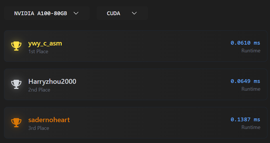
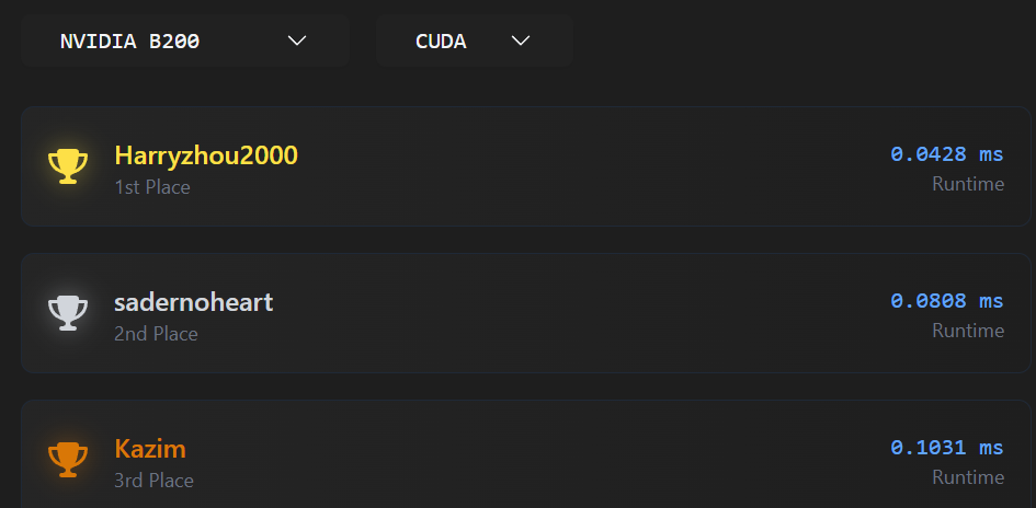
The LeetGPU code

we got second place for A100 and H200 and first place on B200 with this code… it should be only 1/3 of CUBLAS (with 4096**3 case) on A100

A100 rank B200 rank

Basic definitions

head:

 1
 2
 3
 4
 5
 6
 7
 8
 9
10
11
12
13
14
15
16
17
18
19
20
21
22
23
24
25
26
27
28
29
30
#include <cuda_fp16.h>
#include <cuda_runtime.h>
#include <cstdint>
#include <cstdio>
#include <mma.h>
#include <cuda/pipeline>
using namespace nvcuda;

#define CUDA_CHECK_LAST()                                            \
do {                                                                 \
    cudaError_t err = cudaGetLastError();                             \
    if (err != cudaSuccess) {                                        \
        fprintf(stderr,                                              \
                "CUDA kernel launch error %s:%d: %s\n",              \
                __FILE__, __LINE__, cudaGetErrorString(err));         \
        abort();                                                      \
    }                                                                \
} while (0)

constexpr int cdiv(int a, int b) {return (a + b - 1) / b; }
constexpr int warp_size = 32;
__device__ __forceinline__ constexpr int mat_ind(int i, int j, int cols)
{
    return j + i * cols;
}

__device__ __forceinline__ constexpr int mat_ind_cm(int i, int j, int rows)
{
    return i + j * rows;
}

Tile sizes:

1
2
3
4
constexpr int tm = 4 * 2;
constexpr int tn = 8 * 2;
constexpr int ntm = 4 * 2;
constexpr int ntn = 2 * 2;

We use $4\times 8$ data for each warp loader (logically), and $2\times 2$ warps in the thread block.

The thread blocks logically load $(4\times 2) \times (2 \times 2)$ different tiles.

Guaranteed to be a multiple of $16\times 16$ for the sake of WMMA.

K-direction tile sizes:

1
2
constexpr int tk = 32 / 1;
constexpr int ntk = 1;

Derived sizes:

 1
 2
 3
 4
 5
 6
 7
 8
 9
10
// blocksize to load into shmem 
constexpr int bm = tm * ntm;
constexpr int bn = tn * ntn;
constexpr int bk = tk * ntk;
// shmem leading dimensions, 8x2 = 16 bytes for 128-byte alignment
constexpr int lda_loc = bk + 8;
constexpr int ldb_loc = bn + 8;
constexpr int ldb_loc_cm = bk + 8;
constexpr int ldc_loc = bn + 8;
constexpr dim3 epb_dim(bn, bm);

WMMA’s computing sizes

 1
 2
 3
 4
 5
 6
 7
 8
 9
10
11
12
13
14
15
16
17
18
19
20
21
22
23
// each wmma laucnch
constexpr int wmma_m = 16;
constexpr int wmma_n = 16;
constexpr int wmma_k = 16;
// how many wmmas each direction
constexpr int wmma_warp_tiles_m = bm / wmma_m;
constexpr int wmma_warp_tiles_n = bn / wmma_n;
constexpr int wmma_warp_tiles_k = bk / wmma_k;
static_assert(bm % wmma_m == 0);
static_assert(bn % wmma_n == 0);
static_assert(bk % wmma_k == 0);

constexpr int wmma_warp_tile_size_m = 4;
constexpr int wmma_warps_in_block_m = tm / wmma_warp_tile_size_m;
constexpr int wmma_warps_in_block_n = tn / (warp_size / wmma_warp_tile_size_m);
static_assert(tm % wmma_warp_tile_size_m == 0);
static_assert(tn % (warp_size / wmma_warp_tile_size_m) == 0);

constexpr int wmma_warp_mult_m = wmma_warp_tiles_m / wmma_warps_in_block_m;
constexpr int wmma_warp_mult_n = wmma_warp_tiles_n / wmma_warps_in_block_n;

static_assert(wmma_warp_tiles_m % wmma_warps_in_block_m == 0);
static_assert(wmma_warp_tiles_n % wmma_warps_in_block_n == 0);

HGEMM skeleton

The hgemm kernel:

  1
  2
  3
  4
  5
  6
  7
  8
  9
 10
 11
 12
 13
 14
 15
 16
 17
 18
 19
 20
 21
 22
 23
 24
 25
 26
 27
 28
 29
 30
 31
 32
 33
 34
 35
 36
 37
 38
 39
 40
 41
 42
 43
 44
 45
 46
 47
 48
 49
 50
 51
 52
 53
 54
 55
 56
 57
 58
 59
 60
 61
 62
 63
 64
 65
 66
 67
 68
 69
 70
 71
 72
 73
 74
 75
 76
 77
 78
 79
 80
 81
 82
 83
 84
 85
 86
 87
 88
 89
 90
 91
 92
 93
 94
 95
 96
 97
 98
 99
100
101
102
103
104
105
106
107
108
109
110
111
112
113
114
115
116
117
118
119
120
121
122
123
124
125
126
127
128
129
130
131
132
133
134
135
136
137
138
139
140
141
142
143
144
145
template <bool aligned16 = false>
__global__ void hgemm_wmma_cp_async(const half *__restrict__ A, const half *__restrict__ B, half *__restrict__ C,
                                    int M, int N, int K, float alpha, float beta)
{
    // the pipeline here is only single-threaded barrier
    auto pipeline = cuda::make_pipeline();
    const int tid = threadIdx.x + blockDim.x * threadIdx.y;
    const int i_loc = threadIdx.y;
    const int j_loc = threadIdx.x;
    const int i_0 = blockIdx.y * (bm);
    const int j_0 = blockIdx.x * (bn);

    alignas(16) __shared__ half local_A[2][bm * lda_loc];
    alignas(16) __shared__ half local_B[2][bk * ldb_loc];
    alignas(16) __shared__ float local_C[bm * ldc_loc];

    const int warp_id = tid / warp_size;
    const int warp_i = warp_id / wmma_warps_in_block_n;
    const int warp_j = warp_id % wmma_warps_in_block_n;
    //! wrong!
    // const int warp_i = threadIdx.y / wmma_wrap_tile_size_m;
    // const int warp_j = threadIdx.x / (warp_size/ wmma_wrap_tile_size_m);

    // multiple registers at once
    wmma::fragment<
        wmma::accumulator,
        wmma_m, wmma_n, wmma_k,
        float>
        c_frag[wmma_warp_mult_m][wmma_warp_mult_n];
    for (int i = 0; i < wmma_warp_mult_m; i++)
        for (int j = 0; j < wmma_warp_mult_n; j++)
            wmma::fill_fragment(c_frag[i][j], 0.0f);

    int iBuf = 0;
    // load first
    load_matrix_half<bm, bk, bm, bk, lda_loc, MatOrder::rowMajor, aligned16, true>(A, local_A[iBuf],
                                                                                   i_0, 0, 0, 0,
                                                                                   M, K, K /*lda*/,
                                                                                   pipeline);

    load_matrix_half<bk, bn, bk, bn, ldb_loc, MatOrder::rowMajor, aligned16, true>(B, local_B[iBuf],
                                                                                   0, j_0, 0, 0,
                                                                                   K, N, N /*ldb*/,
                                                                                   pipeline);
    // cp_async_commit_group();
    pipeline.producer_commit();

    for (int k_0 = 0; k_0 < K; k_0 += bk)
    {
        if (k_0 + bk < K)
        {
            // load next
            pipeline.producer_acquire();
            load_matrix_half<bm, bk, bm, bk, lda_loc, MatOrder::rowMajor, aligned16, true>(A, local_A[1 - iBuf],
                                                                                           i_0, k_0 + bk, 0, 0,
                                                                                           M, K, K /*lda*/,
                                                                                   pipeline
            );

            load_matrix_half<bk, bn, bk, bn, ldb_loc, MatOrder::rowMajor, aligned16, true>(B, local_B[1 - iBuf],
                                                                                           k_0 + bk, j_0, 0, 0,
                                                                                           K, N, N /*ldb*/,
                                                                                   pipeline
            );
            pipeline.producer_commit();
            // cp_async_commit_group();
            // cp_async_wait_group1();
        }
        // else
        //     cp_async_wait_group0();

        pipeline.consumer_wait();
        __syncthreads();

        if constexpr (!aligned16) // if not aligned, must have
        {
            load_matrix_half_cp_async_ragged_epi<bm, bk, bm, bk, lda_loc>(
                local_A[iBuf],
                i_0, k_0, 0, 0,
                M, K, K);
            load_matrix_half_cp_async_ragged_epi<bk, bn, bk, bn, ldb_loc>(
                local_B[iBuf],
                k_0, j_0, 0, 0,
                K, N, N);
            __syncthreads();
        }
        wmma::fragment<
            wmma::matrix_a,
            wmma_m, wmma_n, wmma_k,
            half,
            wmma::row_major>
            a_frag;
        wmma::fragment<
            wmma::matrix_b,
            wmma_m, wmma_n, wmma_k,
            half,
            wmma::row_major>
            b_frag;

#pragma unroll
        for (int warp_k0_loc = 0; warp_k0_loc < bk; warp_k0_loc += wmma_k)
#pragma unroll
            for (int iW = 0; iW < wmma_warp_mult_m; iW++)
#pragma unroll
                for (int jW = 0; jW < wmma_warp_mult_n; jW++)
                {
                    const int warp_i0_loc = (warp_i + iW * wmma_warps_in_block_m) * wmma_m;
                    const int warp_j0_loc = (warp_j + jW * wmma_warps_in_block_n) * wmma_n;
                    wmma::load_matrix_sync(
                        a_frag,
                        local_A[iBuf] + mat_ind(warp_i0_loc, warp_k0_loc, lda_loc),
                        lda_loc);
                    wmma::load_matrix_sync(
                        b_frag,
                        local_B[iBuf] + mat_ind(warp_k0_loc, warp_j0_loc, ldb_loc),
                        ldb_loc);
                    wmma::mma_sync(c_frag[iW][jW], a_frag, b_frag, c_frag[iW][jW]);
                }
        
        pipeline.consumer_release();
        __syncthreads(); //! barrier here for the input is immediately used as receive field
        iBuf = 1 - iBuf;
    }
    // store C to shmem
    for (int iW = 0; iW < wmma_warp_mult_m; iW++)
        for (int jW = 0; jW < wmma_warp_mult_n; jW++)
        {
            const int warp_i0_loc = (warp_i + iW * wmma_warps_in_block_m) * wmma_m;
            const int warp_j0_loc = (warp_j + jW * wmma_warps_in_block_n) * wmma_n;
            wmma::store_matrix_sync(
                local_C + mat_ind(warp_i0_loc, warp_j0_loc, ldc_loc /*ldc_loc*/),
                c_frag[iW][jW],
                ldc_loc /*ldc_loc*/,
                wmma::mem_row_major);
        }
    __syncthreads();

    

    store_matrix_float_to_half_acc<bm, bn, bm, bn>(C, local_C, alpha, beta,
                                                   i_0, j_0, 0, 0,
                                                   M, N,
                                                   N /*ldc*/, ldc_loc /**/
    );
}

Host driver

Driver code:

 1
 2
 3
 4
 5
 6
 7
 8
 9
10
11
12
extern "C" void solve(const half* A, const half* B, half* C, 
    int M, int N, int K, float alpha, float beta) 
{
    if ((N % 8) == 0 && (K % 8) == 0)// actually lda and ldb
        hgemm_wmma_cp_async</*aligned16=*/true><<<dim3(cdiv(N, epb_dim.x), cdiv(M, epb_dim.y)), tpb_dim>>>(
            A, B, C, M, N, K, alpha, beta 
        );
    else
        hgemm_wmma_cp_async</*aligned16=*/false><<<dim3(cdiv(N, epb_dim.x), cdiv(M, epb_dim.y)), tpb_dim>>>(
            A, B, C, M, N, K, alpha, beta 
        );
}

Async loader

The loading procedure:

 1
 2
 3
 4
 5
 6
 7
 8
 9
10
11
12
13
14
15
16
17
18
19
20
21
22
23
24
25
26
27
28
29
30
31
32
33
34
35
36
37
38
39
40
41
42
43
44
45
46
47
48
49
50
51
52
53
54
55
56
57
58
59
60
61
62
63
64
65
66
67
68
69
70
71
72
73
74
75
76
77
78
79
80
81
82
83
84
85
template<
    int M, int N, 
    int MA_loc, int NA_loc, int ldA_loc,
    MatOrder A_loc_layout = MatOrder::rowMajor,
    bool aligned16 = false,
    bool use_cp_async = false>
__device__ __forceinline__ void load_matrix_half(
    const half* __restrict__ A, half* __restrict__ A_loc,
    int iA, int jA, int iA_loc, int jA_loc, 
    int MA, int NA,
    int ldA,
    cuda::pipeline<cuda::thread_scope_thread> &pipeline)
{
    const int tid = threadIdx.x + blockDim.x * threadIdx.y;
    const int threads_per_block = blockDim.x * blockDim.y;
    static_assert(N % 8 == 0);
    static_assert(ldA_loc % 8 == 0);

    for(int tid0 = 0; tid0  < M * N / 8; tid0 += threads_per_block)
    {
        const int i_ABlk = ((tid + tid0) * 8) / N;
        const int j_ABlk = ((tid + tid0) * 8) % N;
        const int iA_c = iA + i_ABlk;
        const int jA_c = jA + j_ABlk;
        const int iA_loc_c = iA_loc + i_ABlk;
        const int jA_loc_c = jA_loc + j_ABlk;

        if constexpr(!use_cp_async)
        {
            ...
        }
        else
        {
            static_assert(use_cp_async ? A_loc_layout == MatOrder::rowMajor : true);

            if constexpr (aligned16)
            {
                int4 loaded;
                loaded.w = loaded.x = loaded.y = loaded.z = 0;
                if(iA_loc_c < MA_loc && jA_loc_c < NA_loc)
                {
                    if(iA_c < MA && jA_c < NA)
                        cuda::memcpy_async(
                            A_loc + mat_ind(iA_loc_c, jA_loc_c, ldA_loc),
                            A + mat_ind(iA_c, jA_c, ldA),
                            cuda::aligned_size_t<16>(16),
                            pipeline);
                        
                    if(!(iA_c < MA && jA_c < NA))
                        reinterpret_cast<int4*>(A_loc + mat_ind(iA_loc_c, jA_loc_c, ldA_loc))[0] = loaded;
                }
            }
            else //! gets to be ragged
            {
                //! we assuem A itself is aligned
                int left_offset = mat_ind(iA_c, jA_c, ldA) % 8;
                if(iA_loc_c < MA_loc && jA_loc_c < NA_loc)
                {
                    const int cur_ind = mat_ind(iA_c, jA_c, ldA) - left_offset;
                    if(iA_c < MA && jA_c < NA && cur_ind + 7 < MA * ldA)
                        cuda::memcpy_async(
                            A_loc + mat_ind(iA_loc_c, jA_loc_c, ldA_loc),
                            A + mat_ind(iA_c, jA_c - left_offset, ldA), 
                            cuda::aligned_size_t<16>(16),
                            pipeline);

                    if(iA_c < MA && jA_c < NA && cur_ind + 7 >= MA * ldA && cur_ind < MA * ldA)
                        #pragma unroll
                            for(int cur_indd = cur_ind; cur_indd < MA * ldA; cur_indd ++)
                                A_loc[mat_ind(iA_loc_c, jA_loc_c + (cur_indd - cur_ind), ldA_loc)] 
                                    = A[cur_indd];
                    if(jA_loc_c == N - 1) // trailing rag
                    {
                        int j_next = jA_c + 8 - left_offset;
                        if(j_next < NA)
                            #pragma unroll
                            for(int jA_cc = j_next; jA_cc < NA; jA_cc ++)
                                A_loc[mat_ind(iA_loc_c, jA_loc_c + (jA_cc - j_next), ldA_loc)] 
                                    = A[mat_ind(iA_c, jA_cc, ldA)];
                    }
                }
            }
        }
    }
}

For ragged load shifting rows:

 1
 2
 3
 4
 5
 6
 7
 8
 9
10
11
12
13
14
15
16
17
18
19
20
21
22
23
24
25
26
27
28
29
30
31
32
33
34
35
36
37
38
39
40
41
42
43
44
45
template<
    int M, int N, 
    int MA_loc, int NA_loc, int ldA_loc>
__device__ __forceinline__ void load_matrix_half_cp_async_ragged_epi(
    half* __restrict__ A_loc,
    int iA, int jA, int iA_loc, int jA_loc, 
    int MA, int NA,
    int ldA)
{
    // const int i_loc = threadIdx.y;
    // const int j_loc = threadIdx.x;
    const int tid = threadIdx.x + blockDim.x * threadIdx.y;
    const int threads_per_block = blockDim.x * blockDim.y;
    static_assert(N % 8 == 0);
    static_assert(ldA_loc % 8 == 0);

    for(int tid0 = 0; tid0  < M * N / 8; tid0 += threads_per_block)
    {
        const int i_ABlk = ((tid + tid0) * 8) / N;
        const int j_ABlk = ((tid + tid0) * 8) % N;
        const int iA_c = iA + i_ABlk;
        const int jA_c = jA + j_ABlk;
        const int iA_loc_c = iA_loc + i_ABlk;
        const int jA_loc_c = jA_loc + j_ABlk;

        //! we assume A itself is aligned
        int left_offset = mat_ind(iA_c, jA_c, ldA) % 8;
        int4 loaded[16];
        if(iA_loc_c < MA_loc && jA_loc_c < NA_loc)
        {
            loaded[0] = reinterpret_cast<int4*>(A_loc + mat_ind(iA_loc_c, jA_loc_c, ldA_loc))[0];
            loaded[1] = reinterpret_cast<int4*>(A_loc + mat_ind(iA_loc_c, jA_loc_c, ldA_loc))[1];
            for(int i = 0; i < 8; i++)
                reinterpret_cast<half*>(loaded)[i] = reinterpret_cast<half*>(loaded)[i + left_offset]; // shift left;
            if(iA_c >= MA || jA_c >= NA)
                loaded[0].w = loaded[0].x = loaded[0].y = loaded[0].z = 0;
            if(jA_c < NA && jA_c + 7 >= NA)
                for(int jA_cc = jA_c + 7; jA_cc >= NA; jA_cc --)
                    reinterpret_cast<half*>(loaded)[jA_cc - jA_c] = 0.0f;
        }
        __syncthreads();
        if(iA_loc_c < MA_loc && jA_loc_c < NA_loc)
            reinterpret_cast<int4*>(A_loc + mat_ind(iA_loc_c, jA_loc_c, ldA_loc))[0] = loaded[0];
    }
}

Epilogue and store

Store C to global (fused epilogue considering alpha and beta). How to optimize this?

 1
 2
 3
 4
 5
 6
 7
 8
 9
10
11
12
13
14
15
16
17
18
19
20
21
22
23
24
25
26
27
28
29
30
31
32
33
34
35
36
37
38
39
40
41
42
43
44
45
46
47
48
49
50
51
52
53
54
55
56
template<int M, int N, int MA_loc, int NA_loc>
__device__ __forceinline__ void store_matrix_float_to_half_acc(
    half* __restrict__ A, float* __restrict__ A_loc, 
    float alpha, float beta,
    int iA, int jA, int iA_loc, int jA_loc, 
    int MA, int NA,
    int ldA, int ldA_loc)
{
    const int tid = threadIdx.x + blockDim.x * threadIdx.y;
    const int threads_per_block = blockDim.x * blockDim.y;

    static_assert(N % 8 == 0);
    
    for(int tid0 = 0; tid0  < (M * N / 8); tid0 += threads_per_block)
    {
        const int i_ABlk = ((tid + tid0) * 8) / N;
        const int j_ABlk = ((tid + tid0) * 8) % N;
        const int iA_c = iA + i_ABlk;
        const int jA_c = jA + j_ABlk;
        const int iA_loc_c = iA_loc + i_ABlk;
        const int jA_loc_c = jA_loc + j_ABlk;
        if(iA_loc_c < MA_loc && jA_loc_c < NA_loc)
        {
            
            int4 loaded;
            loaded.w = loaded.x = loaded.y = loaded.z = 0;

            if(iA_c < MA)
            {
                if (jA_c + 7 < NA)
                    loaded = reinterpret_cast<const int4*>(A + mat_ind(iA_c, jA_c, ldA))[0];
                else
#pragma unroll
                    for(int jA_cc = jA_c; jA_cc < NA; jA_cc ++)
                        reinterpret_cast<half*>(&loaded)[jA_cc - jA_c] = A[mat_ind(iA_c, jA_cc, ldA)];
            }
#pragma unroll
            for(int i = 0; i < 8; i++)
            {
                float add = A_loc[mat_ind(iA_loc_c, jA_loc_c + i, ldA_loc)] * alpha;
                float old = float(reinterpret_cast<half*>(&loaded)[i]) * beta;
                reinterpret_cast<half*>(&loaded)[i] = old + add;
            }

            if(iA_c < MA)
            {
                if (jA_c + 7 < NA)
                    reinterpret_cast<int4*>(A + mat_ind(iA_c, jA_c, ldA))[0] = loaded;
                else
#pragma unroll
                    for(int jA_cc = jA_c; jA_cc < NA; jA_cc ++)
                        A[mat_ind(iA_c, jA_cc, ldA)] = reinterpret_cast<half*>(&loaded)[jA_cc - jA_c];
            }
        }
    }
}

This store_matrix_float_to_half_acc has bug: the scenario when ldc (lda in the args) unaligned not considered, causes CUDA alignment error.

Streams & Graph

A CUDA stream is a queue of operations (kernel launches, memcpys, events) that:

Execute in issue order within the same stream
May execute concurrently with other streams (if hardware allows)

Default stream

0 or cudaStreamDefault
Historically synchronizes with all other streams (legacy behavior)
Modern CUDA supports per-thread default stream (PTDS)

1
2
3
4
cudaStream_t s;
cudaStreamCreate(&s);
kernel<<<grid, block, 0, s>>>(args...);
cudaStreamDestroy(s);

1
2
cudaMemcpyAsync(dst, src, bytes, cudaMemcpyDeviceToHost, s);
cudaMemsetAsync(ptr, value, bytes, s);

Stream Synchronization

1
cudaStreamSynchronize(s1);

Blocks host
Heavy hammer
Avoid in performance-critical paths

Stream Events

Record an event

1
2
3
cudaEvent_t e;
cudaEventCreate(&e);
cudaEventRecord(e, s1);

Make another stream wait

1
cudaStreamWaitEvent(s2, e, 0);

Result

1
2
s1:  kernelA → event
s2:                wait → kernelB

No host blocking
The dependency is like inserted into the queues.

Event Sync

1
cudaEventSynchronize(e);

Used when correctness requires host visibility.

A CUDA graph is:

A static DAG of GPU operations captured once and replayed many times

Kernel launch overhead is non-trivial
Repeated patterns are common (CFD timesteps, solvers)
Graph replay is much cheaper than re-launching kernels

Nodes can be:

Kernel launches
Memcpy / memset
Host functions
Event record / wait
Child graphs

Graph Construction: Stream capture

1
2
3
4
5
6
7
cudaStreamBeginCapture(s, cudaStreamCaptureModeGlobal);

kernelA<<<..., s>>>();
kernelB<<<..., s>>>();
cudaMemcpyAsync(..., s);

cudaStreamEndCapture(s, &graph);

Then:

1
2
cudaGraphInstantiate(&graphExec, graph, nullptr, nullptr, 0);
cudaGraphLaunch(graphExec, s);

Graph Construction: Manual

1
2
3
4
cudaGraphCreate(&graph, 0);

cudaGraphAddKernelNode(&nodeA, graph, nullptr, 0, &paramsA);
cudaGraphAddKernelNode(&nodeB, graph, &nodeA, 1, &paramsB);

CUDA Performance Analysis

About the GEMM + nsight compute:

1
sudo /usr/local/cuda-12.6/bin/ncu --set roofline --target-processes all ./hgemmLearn.exe

Shows:

1
2
3
4
5
6
7
8
==PROF== Profiling "hgemm_wmma_cp_async" - 0: 0%....50%....100% - 15 passes
==PROF== Profiling "ampere_fp16_s16816gemm_fp16_2..." - 1: 0%....50%....100% - 15 passe
==PROF== Profiling "hgemm_wmma_cp_async" - 2: 0%....50%....100% - 15 passes
==PROF== Profiling "hgemm_wmma_cp_async" - 3: 0%....50%....100% - 15 passes
==PROF== Profiling "hgemm_wmma_cp_async" - 4: 0%....50%....100% - 15 passes
==PROF== Profiling "ampere_fp16_s16816gemm_fp16_2..." - 5: 0%....50%....100% - 15 passes
==PROF== Profiling "ampere_fp16_s16816gemm_fp16_2..." - 6: 0%....50%....100% - 15 passes
==PROF== Profiling "ampere_fp16_s16816gemm_fp16_2..." - 7: 0%....50%....100% - 15 passes

For once of hgemm_wmma_cp_async, results:

 1
 2
 3
 4
 5
 6
 7
 8
 9
10
11
12
13
14
15
16
17
18
19
20
21
22
23
24
25
26
27
28
29
30
31
32
33
34
35
36
37
38
39
40
41
42
43
44
45
46
47
48
49
50
51
52
53
54
55
56
57
58
59
60
61
62
63
64
65
66
67
68
69
70
71
72
73
74
75
76
77
78
79
80
81
82
83
  void hgemm_wmma_cp_async<1>(const __half *, const __half *, __half *, int, int, int, float, float) (64, 64, 1)x(16, 8, 1), Context 1, Stream 7, Device 0, CC 8.0
    Section: GPU Speed Of Light Throughput
    ----------------------- ----------- ------------
    Metric Name             Metric Unit Metric Value
    ----------------------- ----------- ------------
    DRAM Frequency                  Ghz         1.51
    SM Frequency                    Ghz         1.06
    Elapsed Cycles                cycle    2,339,707
    Memory Throughput                 %        73.10
    DRAM Throughput                   %        17.07
    Duration                         ms         2.20
    L1/TEX Cache Throughput           %        74.07
    L2 Cache Throughput               %        68.11
    SM Active Cycles              cycle 2,296,883.04
    Compute (SM) Throughput           %        53.53
    ----------------------- ----------- ------------

    OPT   Memory is more heavily utilized than Compute: Look at the Memory Workload Analysis section to identify the L1 
          bottleneck. Check memory replay (coalescing) metrics to make sure you're efficiently utilizing the bytes      
          transferred. Also consider whether it is possible to do more work per memory access (kernel fusion) or        
          whether there are values you can (re)compute.                                                                 

    Section: GPU Speed Of Light Roofline Chart
    INF   The ratio of peak float (fp32) to double (fp64) performance on this device is 2:1. The kernel achieved  close 
          to 0% of this device's fp32 peak performance and 0% of its fp64 peak performance. See the Kernel Profiling    
          Guide (https://docs.nvidia.com/nsight-compute/ProfilingGuide/index.html#roofline) for more details on         
          roofline analysis.                                                                                            

    Section: Scheduler Statistics
    ---------------------------- ----------- ------------
    Metric Name                  Metric Unit Metric Value
    ---------------------------- ----------- ------------
    One or More Eligible                   %        54.31
    Issued Warp Per Scheduler                        0.54
    No Eligible                            %        45.69
    Active Warps Per Scheduler          warp         3.88
    Eligible Warps Per Scheduler        warp         0.87
    ---------------------------- ----------- ------------

    OPT   Est. Local Speedup: 26.9%                                                                                     
          Every scheduler is capable of issuing one instruction per cycle, but for this kernel each scheduler only      
          issues an instruction every 1.8 cycles. This might leave hardware resources underutilized and may lead to     
          less optimal performance. Out of the maximum of 16 warps per scheduler, this kernel allocates an average of   
          3.88 active warps per scheduler, but only an average of 0.87 warps were eligible per cycle. Eligible warps    
          are the subset of active warps that are ready to issue their next instruction. Every cycle with no eligible   
          warp results in no instruction being issued and the issue slot remains unused. To increase the number of      
          eligible warps, avoid possible load imbalances due to highly different execution durations per warp.          
          Reducing stalls indicated on the Warp State Statistics and Source Counters sections can help, too.            

    Section: Occupancy
    ------------------------------- ----------- ------------
    Metric Name                     Metric Unit Metric Value
    ------------------------------- ----------- ------------
    Block Limit SM                        block           32
    Block Limit Registers                 block            8
    Block Limit Shared Mem                block            4
    Block Limit Warps                     block           16
    Theoretical Active Warps per SM        warp           16
    Theoretical Occupancy                     %           25
    Achieved Occupancy                        %        24.22
    Achieved Active Warps Per SM           warp        15.50
    ------------------------------- ----------- ------------

    OPT   Est. Speedup: 26.9%                                                                                           
          The 4.00 theoretical warps per scheduler this kernel can issue according to its occupancy are below the       
          hardware maximum of 16. This kernel's theoretical occupancy (25.0%) is limited by the required amount of      
          shared memory.                                                                                                

    Section: GPU and Memory Workload Distribution
    -------------------------- ----------- -------------
    Metric Name                Metric Unit  Metric Value
    -------------------------- ----------- -------------
    Average DRAM Active Cycles       cycle    567,450.60
    Total DRAM Elapsed Cycles        cycle   132,935,680
    Average L1 Active Cycles         cycle  2,296,883.04
    Total L1 Elapsed Cycles          cycle   251,341,852
    Average L2 Active Cycles         cycle  2,213,460.11
    Total L2 Elapsed Cycles          cycle   179,234,000
    Average SM Active Cycles         cycle  2,296,883.04
    Total SM Elapsed Cycles          cycle   251,341,852
    Average SMSP Active Cycles       cycle  2,293,731.12
    Total SMSP Elapsed Cycles        cycle 1,005,367,408
    -------------------------- ----------- -------------

The cuBLAS result:

  1
  2
  3
  4
  5
  6
  7
  8
  9
 10
 11
 12
 13
 14
 15
 16
 17
 18
 19
 20
 21
 22
 23
 24
 25
 26
 27
 28
 29
 30
 31
 32
 33
 34
 35
 36
 37
 38
 39
 40
 41
 42
 43
 44
 45
 46
 47
 48
 49
 50
 51
 52
 53
 54
 55
 56
 57
 58
 59
 60
 61
 62
 63
 64
 65
 66
 67
 68
 69
 70
 71
 72
 73
 74
 75
 76
 77
 78
 79
 80
 81
 82
 83
 84
 85
 86
 87
 88
 89
 90
 91
 92
 93
 94
 95
 96
 97
 98
 99
100
101
102
103
104
105
106
107
108
109
110
111
112
113
114
115
116
117
118
119
120
121
122
123
124
125
126
127
128
129
130
131
132
133
134
135
136
137
138
139
140
141
142
143
144
145
146
147
148
149
150
151
152
153
154
155
156
157
158
159
160
161
162
163
164
165
166
167
168
169
170
171
172
173
174
175
176
177
178
179
180
181
182
183
184
185
186
187
188
189
190
191
  ampere_fp16_s16816gemm_fp16_256x128_ldg8_f2f_stages_32x3_nn (16, 32, 1)x(256, 1, 1), Context 1, Stream 7, Device 0, CC 8.0
    Section: GPU Speed Of Light Throughput
    ----------------------- ----------- ------------
    Metric Name             Metric Unit Metric Value
    ----------------------- ----------- ------------
    DRAM Frequency                  Ghz         1.51
    SM Frequency                    Ghz         1.06
    Elapsed Cycles                cycle      707,205
    Memory Throughput                 %        47.32
    DRAM Throughput                   %        15.42
    Duration                         us       665.15
    L1/TEX Cache Throughput           %        50.19
    L2 Cache Throughput               %        46.49
    SM Active Cycles              cycle   666,468.55
    Compute (SM) Throughput           %        87.92
    ----------------------- ----------- ------------

    INF   The kernel is utilizing greater than 80.0% of the available compute or memory performance of the device. To   
          further improve performance, work will likely need to be shifted from the most utilized to another unit.      
          Start by analyzing workloads in the Compute Workload Analysis section.                                        

    Section: GPU Speed Of Light Roofline Chart
    INF   The ratio of peak float (fp32) to double (fp64) performance on this device is 2:1. The kernel achieved  close 
          to 0% of this device's fp32 peak performance and 0% of its fp64 peak performance. See the Kernel Profiling    
          Guide (https://docs.nvidia.com/nsight-compute/ProfilingGuide/index.html#roofline) for more details on         
          roofline analysis.                                                                                            

    Section: Scheduler Statistics
    ---------------------------- ----------- ------------
    Metric Name                  Metric Unit Metric Value
    ---------------------------- ----------- ------------
    One or More Eligible                   %        21.34
    Issued Warp Per Scheduler                        0.21
    No Eligible                            %        78.66
    Active Warps Per Scheduler          warp         2.00
    Eligible Warps Per Scheduler        warp         0.33
    ---------------------------- ----------- ------------

    OPT   Est. Local Speedup: 12.08%                                                                                    
          Every scheduler is capable of issuing one instruction per cycle, but for this kernel each scheduler only      
          issues an instruction every 4.7 cycles. This might leave hardware resources underutilized and may lead to     
          less optimal performance. Out of the maximum of 16 warps per scheduler, this kernel allocates an average of   
          2.00 active warps per scheduler, but only an average of 0.33 warps were eligible per cycle. Eligible warps    
          are the subset of active warps that are ready to issue their next instruction. Every cycle with no eligible   
          warp results in no instruction being issued and the issue slot remains unused. To increase the number of      
          eligible warps, avoid possible load imbalances due to highly different execution durations per warp.          
          Reducing stalls indicated on the Warp State Statistics and Source Counters sections can help, too.            

    Section: Occupancy
    ------------------------------- ----------- ------------
    Metric Name                     Metric Unit Metric Value
    ------------------------------- ----------- ------------
    Block Limit SM                        block           32
    Block Limit Registers                 block            1
    Block Limit Shared Mem                block            1
    Block Limit Warps                     block            8
    Theoretical Active Warps per SM        warp            8
    Theoretical Occupancy                     %        12.50
    Achieved Occupancy                        %        12.49
    Achieved Active Warps Per SM           warp         8.00
    ------------------------------- ----------- ------------

    OPT   Est. Speedup: 12.08%                                                                                          
          The 2.00 theoretical warps per scheduler this kernel can issue according to its occupancy are below the       
          hardware maximum of 16. This kernel's theoretical occupancy (12.5%) is limited by the number of required      
          registers. This kernel's theoretical occupancy (12.5%) is limited by the required amount of shared memory.    

    Section: GPU and Memory Workload Distribution
    -------------------------- ----------- ------------
    Metric Name                Metric Unit Metric Value
    -------------------------- ----------- ------------
    Average DRAM Active Cycles       cycle   155,022.60
    Total DRAM Elapsed Cycles        cycle   40,223,744
    Average L1 Active Cycles         cycle   666,468.55
    Total L1 Elapsed Cycles          cycle   76,331,900
    Average L2 Active Cycles         cycle   667,506.90
    Total L2 Elapsed Cycles          cycle   54,153,440
    Average SM Active Cycles         cycle   666,468.55
    Total SM Elapsed Cycles          cycle   76,331,900
    Average SMSP Active Cycles       cycle   666,237.23
    Total SMSP Elapsed Cycles        cycle  305,327,600
    -------------------------- ----------- ------------

    OPT   Est. Speedup: 5.012%                                                                                          
          One or more SMs have a much lower number of active cycles than the average number of active cycles. Maximum   
          instance value is 5.31% above the average, while the minimum instance value is 15.63% below the average.      
    ----- --------------------------------------------------------------------------------------------------------------
    OPT   Est. Speedup: 5.012%                                                                                          
          One or more SMSPs have a much lower number of active cycles than the average number of active cycles. Maximum 
          instance value is 5.32% above the average, while the minimum instance value is 15.84% below the average.      
    ----- --------------------------------------------------------------------------------------------------------------
    OPT   Est. Speedup: 5.012%                                                                                          
          One or more L1 Slices have a much lower number of active cycles than the average number of active cycles.     
          Maximum instance value is 5.31% above the average, while the minimum instance value is 15.63% below the       
          average.                                                                                                      

  ampere_fp16_s16816gemm_fp16_256x128_ldg8_f2f_stages_32x3_nn (16, 32, 1)x(256, 1, 1), Context 1, Stream 7, Device 0, CC 8.0
    Section: GPU Speed Of Light Throughput
    ----------------------- ----------- ------------
    Metric Name             Metric Unit Metric Value
    ----------------------- ----------- ------------
    DRAM Frequency                  Ghz         1.51
    SM Frequency                    Ghz         1.06
    Elapsed Cycles                cycle      707,405
    Memory Throughput                 %        47.34
    DRAM Throughput                   %        15.38
    Duration                         us       666.62
    L1/TEX Cache Throughput           %        50.18
    L2 Cache Throughput               %        46.53
    SM Active Cycles              cycle   666,456.30
    Compute (SM) Throughput           %        87.95
    ----------------------- ----------- ------------

    INF   The kernel is utilizing greater than 80.0% of the available compute or memory performance of the device. To   
          further improve performance, work will likely need to be shifted from the most utilized to another unit.      
          Start by analyzing workloads in the Compute Workload Analysis section.                                        

    Section: GPU Speed Of Light Roofline Chart
    INF   The ratio of peak float (fp32) to double (fp64) performance on this device is 2:1. The kernel achieved  close 
          to 0% of this device's fp32 peak performance and 0% of its fp64 peak performance. See the Kernel Profiling    
          Guide (https://docs.nvidia.com/nsight-compute/ProfilingGuide/index.html#roofline) for more details on         
          roofline analysis.                                                                                            

    Section: Scheduler Statistics
    ---------------------------- ----------- ------------
    Metric Name                  Metric Unit Metric Value
    ---------------------------- ----------- ------------
    One or More Eligible                   %        21.34
    Issued Warp Per Scheduler                        0.21
    No Eligible                            %        78.66
    Active Warps Per Scheduler          warp         2.00
    Eligible Warps Per Scheduler        warp         0.33
    ---------------------------- ----------- ------------

    OPT   Est. Local Speedup: 12.05%                                                                                    
          Every scheduler is capable of issuing one instruction per cycle, but for this kernel each scheduler only      
          issues an instruction every 4.7 cycles. This might leave hardware resources underutilized and may lead to     
          less optimal performance. Out of the maximum of 16 warps per scheduler, this kernel allocates an average of   
          2.00 active warps per scheduler, but only an average of 0.33 warps were eligible per cycle. Eligible warps    
          are the subset of active warps that are ready to issue their next instruction. Every cycle with no eligible   
          warp results in no instruction being issued and the issue slot remains unused. To increase the number of      
          eligible warps, avoid possible load imbalances due to highly different execution durations per warp.          
          Reducing stalls indicated on the Warp State Statistics and Source Counters sections can help, too.            

    Section: Occupancy
    ------------------------------- ----------- ------------
    Metric Name                     Metric Unit Metric Value
    ------------------------------- ----------- ------------
    Block Limit SM                        block           32
    Block Limit Registers                 block            1
    Block Limit Shared Mem                block            1
    Block Limit Warps                     block            8
    Theoretical Active Warps per SM        warp            8
    Theoretical Occupancy                     %        12.50
    Achieved Occupancy                        %        12.49
    Achieved Active Warps Per SM           warp         8.00
    ------------------------------- ----------- ------------

    OPT   Est. Speedup: 12.05%                                                                                          
          The 2.00 theoretical warps per scheduler this kernel can issue according to its occupancy are below the       
          hardware maximum of 16. This kernel's theoretical occupancy (12.5%) is limited by the number of required      
          registers. This kernel's theoretical occupancy (12.5%) is limited by the required amount of shared memory.    

    Section: GPU and Memory Workload Distribution
    -------------------------- ----------- ------------
    Metric Name                Metric Unit Metric Value
    -------------------------- ----------- ------------
    Average DRAM Active Cycles       cycle   155,059.60
    Total DRAM Elapsed Cycles        cycle   40,314,880
    Average L1 Active Cycles         cycle   666,456.30
    Total L1 Elapsed Cycles          cycle   76,300,864
    Average L2 Active Cycles         cycle   668,507.29
    Total L2 Elapsed Cycles          cycle   54,106,080
    Average SM Active Cycles         cycle   666,456.30
    Total SM Elapsed Cycles          cycle   76,300,864
    Average SMSP Active Cycles       cycle   666,170.74
    Total SMSP Elapsed Cycles        cycle  305,203,456
    -------------------------- ----------- ------------

    OPT   Est. Speedup: 5.039%                                                                                          
          One or more SMs have a much lower number of active cycles than the average number of active cycles. Maximum   
          instance value is 5.34% above the average, while the minimum instance value is 15.93% below the average.      
    ----- --------------------------------------------------------------------------------------------------------------
    OPT   Est. Speedup: 5.034%                                                                                          
          One or more SMSPs have a much lower number of active cycles than the average number of active cycles. Maximum 
          instance value is 5.34% above the average, while the minimum instance value is 15.82% below the average.      
    ----- --------------------------------------------------------------------------------------------------------------
    OPT   Est. Speedup: 5.039%                                                                                          
          One or more L1 Slices have a much lower number of active cycles than the average number of active cycles.     
          Maximum instance value is 5.34% above the average, while the minimum instance value is 15.93% below the       
          average.                                                                                                      

MPI

Great target 👍 — for NVIDIA Developer Technology (DevTech) Intern, especially a system-level performance optimization role, MPI questions usually focus less on “write MPI from scratch” and more on performance reasoning, communication patterns, and interaction with GPUs / systems. Given your CFD + MPI background, you’re actually very well aligned.

Below is a structured list of common MPI interview questions, grouped by theme, with brief hints on what the interviewer usually wants to hear.

1. MPI Fundamentals (Warm-up / Sanity Check)

These verify you truly understand MPI beyond syntax.

What is MPI and why is it used instead of shared memory?
- Distributed memory model
- Scalability, portability, performance control
Difference between MPI_Send and MPI_Isend?
- Blocking vs non-blocking
- Progress, overlap, completion semantics
What does MPI_Init / MPI_Finalize do?
- Process environment setup, communicator creation
What is a communicator?
- MPI_COMM_WORLD
- Context + group
- Why communicators matter for correctness and performance
Difference between rank and size?
- MPI_Comm_rank, MPI_Comm_size
What happens if one rank does not call a collective?
- Deadlock / undefined behavior

2. Point-to-Point Communication (Very Common)

These often appear with deadlock or performance reasoning.

Explain eager vs rendezvous protocol
- Message size threshold
- Buffering vs handshake
- Why large messages can deadlock
Can MPI_Send deadlock? Give an example
- Symmetric sends without matching receives
- Depends on message size / buffering
Difference between MPI_Isend + MPI_Wait vs MPI_Send
- Overlap potential
- Need to manage request lifetime
What does MPI_Probe do? When would you use it?

Unknown message size
Dynamic communication patterns

What is message matching in MPI?

(source, tag, communicator)
Why incorrect tags cause bugs

3. Collectives

Expect performance-oriented questions here.

Difference between MPI_Bcast, MPI_Scatter, MPI_Gather, MPI_Allgather

Communication patterns
Use cases in CFD / AI

What is MPI_Reduce vs MPI_Allreduce?

Rooted vs replicated result
Cost difference

Why is MPI_Allreduce often a bottleneck?

Global synchronization
Latency-dominated
Scaling issues

How is MPI_Allreduce typically implemented?

Tree-based
Ring
Rabenseifner
Topology-aware algorithms

When would you replace collectives with point-to-point?

Irregular communication
Partial participation
Avoid global sync

4. Performance & Scalability (Very Likely)

This is core DevTech territory.

Strong scaling vs weak scaling

Fixed problem size vs fixed work per rank

Why does MPI performance degrade at high core counts?

Latency domination
Network contention
Synchronization
Load imbalance

What is communication–computation overlap?

Non-blocking communication
Progress engines
Practical limitations

How do you identify MPI bottlenecks?

Profilers: Nsight Systems, VTune, mpiP
Time in collectives
Idle time / imbalance

What is Amdahl’s Law vs Gustafson’s Law?

Strong vs weak scaling interpretation

\[ S(N) = \frac{1}{(1 - P) + \frac{P}{N}} \]\[ S(N) = N - (1 - P)(N - 1) \]

5. MPI + System Architecture (NUMA / Network)

NVIDIA loves system-level awareness.

What is NUMA and why does it matter for MPI?

Memory locality
Rank placement
First-touch policy

How does process binding affect MPI performance?

Core affinity
Cache reuse
Avoid oversubscription

What is network topology awareness?

Fat-tree vs dragonfly
Intra-node vs inter-node communication

Difference between intra-node and inter-node MPI communication

Shared memory vs network
Latency and bandwidth

6. MPI + GPU (Very Important for NVIDIA)

Even if you’re not a CUDA expert yet, expect these.

What is CUDA-aware MPI?

GPU pointers passed directly to MPI
Avoid host staging

How does GPU–GPU communication work across nodes?

GPUDirect RDMA
NIC ↔ GPU memory

What are the benefits of CUDA-aware MPI?

Lower latency
Higher bandwidth
Less CPU involvement

How would you overlap MPI communication with GPU kernels?

CUDA streams
Non-blocking MPI
Events for synchronization

What happens if MPI is not CUDA-aware?

Explicit cudaMemcpy
Extra synchronization
Performance penalty

7. CFD-Style MPI Questions (Your Advantage)

Interviewers often probe domain intuition.

How is MPI typically used in CFD solvers?

Domain decomposition
Halo / ghost cell exchange
Reductions for residuals

Why are halo exchanges latency-sensitive?

Small messages
Frequent synchronization

How would you optimize halo exchange?

Non-blocking communication
Packing
Neighborhood collectives
Overlap with interior computation

What MPI pattern dominates CFD time-to-solution?

Nearest-neighbor communication
Global reductions

8. Debugging & Correctness

Often mixed with performance.

Common MPI bugs you’ve seen

Deadlocks
Mismatched collectives
Tag mismatches
Incorrect buffer lifetimes

How do you debug MPI deadlocks?

Print rank-tag tracing
Reduce to 2–4 ranks
Use MPI correctness tools

RDMA ?

NCCL

Basics

1. Communicator

A communicator defines:

Which GPUs participate
Their ranks
Their topology

Created once, reused across iterations:

1
ncclCommInitRank(...)

At system level:

Expensive → cache it
Initialization cost matters for short jobs

2. AllReduce (core AI primitive)

Used for:

Gradient synchronization
Model parameter aggregation

Mathematically:

1
2
Each GPU has X
All GPUs get sum(X) / or sum(X)

NCCL implements ring, tree, or hybrid algorithms depending on:

Message size
Topology
Number of GPUs

3. Topology awareness (very important)

NCCL discovers system topology at runtime:

GPU ↔ GPU (NVLink, PCIe)
GPU ↔ NIC (NVLink-NIC, PCIe switch)
NUMA domains

It builds communication rings/trees that:

Prefer NVLink over PCIe
Minimize PCIe root crossings
Optimize NIC usage

👉 Bad topology → bad scaling

4. Intra-node vs Inter-node NCCL

Intra-node

NVLink / PCIe
Very high bandwidth, low latency
Typically near-ideal scaling

Inter-node

Uses:
- InfiniBand (RDMA)
- Ethernet (RoCE)
GPU Direct RDMA (GDR) if enabled

Key system-level factors:

NIC placement
GPU-NIC affinity
NUMA alignment

5. GPU Direct RDMA (GDR)

Allows:

1
2
GPU memory ↔ NIC
(no host memory bounce)

Benefits:

Lower latency
Higher bandwidth
Less CPU overhead

System requirements:

Supported NIC (e.g. Mellanox)
Correct driver stack
IOMMU / ACS settings matter

NCCL execution model

NCCL calls are asynchronous
Enqueued into a CUDA stream
Synchronization happens via:
- CUDA events
- Stream waits

Example (conceptual):

1
2
ncclAllReduce(..., stream);
cudaKernel<<<..., stream>>>();

👉 Enables communication–computation overlap

NCCL in AI frameworks

PyTorch

Uses NCCL backend for DistributedDataParallel
One NCCL communicator per process group
Gradient buckets → AllReduce

Performance knobs:

Bucket size
Overlap on/off
Stream usage

Multi-node training stack

Typical flow:

1
2
3
4
5
6
7
SLURM / mpirun
↓
1 process per GPU
↓
NCCL communicators
↓
CUDA streams

MPI is often used only for:

Rank assignment
Environment setup

Common system-level performance issues

1. Wrong GPU–NIC affinity

Symptoms:

Low bandwidth
Unbalanced traffic

Fix:

Bind processes correctly
Match GPU closest to NIC

2. NUMA misalignment

Symptoms:

High CPU usage
Inconsistent iteration time

Fix:

CPU pinning
Correct process placement

3. Oversubscription

Too many processes per socket
Competes for PCIe / memory bandwidth

4. Small message sizes

NCCL bandwidth not saturated
Ring startup dominates

Common in:

Small models
Too many gradient buckets

NCCL APIs

1. Communicator & Initialization APIs

These define who participates in collectives.

Core communicator APIs

1
2
3
4
5
ncclGetUniqueId(ncclUniqueId* id);
ncclCommInitRank(ncclComm_t* comm,
                 int nranks,
                 ncclUniqueId id,
                 int rank);

ncclGetUniqueId Generates a unique ID (usually on rank 0, broadcast via MPI)
ncclCommInitRank Creates a communicator for one rank

📌 System-level note

Communicator creation is expensive
Should be done once, reused across iterations

Multi-GPU per process

1
2
3
ncclCommInitAll(ncclComm_t* comms,
                int ndev,
                const int* devlist);

Used when one process controls multiple GPUs
Common in single-node setups

Communicator teardown

1
ncclCommDestroy(ncclComm_t comm);

2. Collective Communication APIs (Core NCCL Value)

Most common collectives

1
2
3
4
5
ncclAllReduce(...)
ncclReduce(...)
ncclBroadcast(...)
ncclAllGather(...)
ncclReduceScatter(...)

Full prototype (example: AllReduce)

1
2
3
4
5
6
7
ncclAllReduce(const void* sendbuf,
              void* recvbuf,
              size_t count,
              ncclDataType_t datatype,
              ncclRedOp_t op,
              ncclComm_t comm,
              cudaStream_t stream);

Supported reductions

1
2
3
4
ncclSum
ncclProd
ncclMax
ncclMin

3. Group APIs (Latency Optimization)

Used to batch multiple NCCL calls.

1
2
ncclGroupStart();
ncclGroupEnd();

Example:

1
2
3
4
ncclGroupStart();
ncclAllReduce(..., stream1);
ncclAllReduce(..., stream2);
ncclGroupEnd();

📌 Why this matters

Reduces launch and synchronization overhead
Improves performance when launching many collectives
Common inside DL frameworks

4. CUDA Stream Integration (Critical)

Every collective takes a:

1
cudaStream_t stream

Meaning:

NCCL ops are enqueued, not executed immediately
They respect stream dependencies
They can overlap with computation

Example:

1
2
3
cudaStream_t s;
ncclAllReduce(..., s);
kernel<<<..., s>>>();

5. CUDA Graph Compatibility

NCCL collectives can be captured in CUDA Graphs.

Flow:

1
2
3
4
cudaStreamBeginCapture(stream, ...);
ncclAllReduce(..., stream);
cudaStreamEndCapture(stream, &graph);
cudaGraphInstantiate(&graphExec, graph, ...);

📌 Benefits:

Removes CPU launch overhead
Important for short-iteration AI workloads
Used in high-performance training loops

Point-to-point

NCCL does have point-to-point now.

Since NCCL 2.7+:

1
2
ncclSend()
ncclRecv()

These are:

GPU-to-GPU
CUDA-stream-aware
NVLink / IB optimized

So pipeline parallelism can use:

ncclSend/Recv
CUDA IPC
Or even CUDA memcpy (same node)

How pipeline parallelism is actually implemented

Option 1: NCCL Send / Recv (common today)

Forward:

1
2
3
GPU i:
  compute(layer_i)
  ncclSend(activation → GPU i+1)

Backward:

1
2
3
GPU i:
  ncclRecv(grad → GPU i+1)
  compute_backward(layer_i)

This is streamed, overlappable with compute.

Option 2: CUDA-aware MPI (less common in DL)

Used sometimes for:

Inter-node activation passing
Research frameworks

But:

NCCL is preferred in production DL

Option 3: Collectives (less common for PP)

Some frameworks:

Use AllGather instead of send/recv
Especially when multiple next stages exist

6. Why NCCL collectives still matter in PP

Even in pipeline parallelism:

Phase	Communication
Forward	Send activations
Backward	Send activation gradients
Optimizer	DP AllReduce
TP	AllReduce / ReduceScatter
MoE	AllToAll

LLM

1. System-Level View: What Is an LLM?

At the highest level, a modern LLM is:

A large autoregressive sequence model that predicts the next token, trained on massive corpora, and deployed with aggressive parallelism and memory optimization.

Key properties:

Autoregressive: predict token_t given token_<t
Token-based: text → tokens → embeddings
Scale-driven: performance comes primarily from model/data/compute scaling
GPU-first: designed around dense linear algebra

2. Model Family Level: Transformer-Based Models

Nearly all modern LLMs are based on Transformers, with variations.

Canonical examples

GPT-3/4, LLaMA, Mistral, Qwen → Decoder-only Transformers
PaLM, Gemini → Transformer variants
Mixtral → Mixture-of-Experts Transformer

Why Transformers?

No recurrence → parallelizable
Attention → global context
Works extremely well with matrix multiply accelerators

3. Macro Architecture: Decoder-Only Transformer

Most LLMs you’ll encounter are decoder-only:

 1
 2
 3
 4
 5
 6
 7
 8
 9
10
11
Input Tokens
   ↓
Token Embedding + Positional Encoding
   ↓
[ Transformer Block ] × N
   ↓
LayerNorm
   ↓
Linear Projection → Vocabulary
   ↓
Softmax → Next Token

Important:

No encoder
Causal (masked) attention
Same block repeated N times (e.g., 32–120 layers)

4. Transformer Block Anatomy (Critical)

Each Transformer block consists of:

 1
 2
 3
 4
 5
 6
 7
 8
 9
10
11
12
13
x
│
├─ LayerNorm
│
├─ Multi-Head Self Attention
│
├─ Residual Add
│
├─ LayerNorm
│
├─ Feed Forward Network (MLP)
│
└─ Residual Add

This is where 90%+ of compute happens.

5. Attention Mechanism (The Core Idea)

Scaled Dot-Product Attention

For each token:

1
2
3
4
5
Q = X Wq
K = X Wk
V = X Wv

Attention(Q,K,V) = softmax(QKᵀ / √d) V

Properties:

Quadratic complexity: O(seq²)
Memory heavy (attention matrix)
Dominates inference latency at long context

Causal Masking

Prevents attending to future tokens
Enables autoregressive generation

6. Multi-Head Attention (MHA)

Instead of one attention:

Split into h heads
Each head attends to different subspaces

1
d_model = h × d_head

Benefits:

Better representation
Still maps to GEMMs → GPU-friendly

7. Feed-Forward Network (MLP)

Typical form:

1
FFN(x) = W2 σ(W1 x)

Modern variants:

GELU / SiLU
SwiGLU / GeGLU (used in LLaMA, Mistral)

Key facts:

FFN often costs more FLOPs than attention
Extremely GEMM-heavy
Memory bandwidth sensitive

8. Normalization & Residuals

LayerNorm / RMSNorm

Stabilizes training
RMSNorm removes mean → cheaper

Residual Connections

Enable deep networks
Improve gradient flow
Important for numerical stability

9. Positional Information

Since attention is permutation-invariant, position must be injected.

Common approaches

Absolute embeddings (older)
RoPE (Rotary Positional Embedding) ← dominant today
ALiBi (linear bias)

RoPE:

Enables better extrapolation to long context
Implemented inside Q/K projection

10. Tokenization & Embeddings

Tokenization

BPE / SentencePiece
Subword-based
Vocabulary ~32k–100k

Embedding Layer

Token ID → dense vector
Often tied with output projection weights

11. Training Objective

LLMs are trained with:

1
Cross-Entropy Loss

Objective:

1
maximize log P(token_t | token_<t)

Training:

Teacher forcing
Massive batch sizes
Trillions of tokens

12. Scaling Laws (Why Size Matters)

Empirical laws:

Performance scales smoothly with:
- Model size
- Dataset size
- Compute budget

This motivates:

Bigger models
Better parallelism
Memory optimization

13. Parallelism Strategies (System-Level Critical)

Modern LLMs cannot fit or run on one GPU.

Parallelism types

Data Parallelism (DP)
Tensor Parallelism (TP) – split matrices
Pipeline Parallelism (PP) – split layers
Sequence Parallelism
Expert Parallelism (MoE)

Frameworks:

Megatron-LM
DeepSpeed
FSDP
NCCL underneath all of them

14. Mixture of Experts (MoE)

Instead of dense FFN:

1
Router → select top-k experts → sparse FFN

Benefits:

More parameters
Same compute cost
Harder to scale (communication heavy)

Used in:

Mixtral
Switch Transformer

15. Inference-Time Architecture Changes

KV Cache

Cache K/V from previous tokens
Reduces attention cost from O(T²) → O(T)

Autoregressive Loop

1
2
3
for t in tokens:
  run model
  sample next token

Bottlenecks

Memory bandwidth
Small batch sizes
Kernel launch overhead

16. Performance-Critical Kernels (GPU View)

At the lowest level, everything reduces to:

GEMM
Softmax
LayerNorm
Memory movement

Optimizations:

FlashAttention
Fused kernels
Tensor Cores (FP16 / BF16 / FP8)
CUDA Graphs
NCCL collectives

17. Summary Stack (One Slide Mental Model)

 1
 2
 3
 4
 5
 6
 7
 8
 9
10
11
12
13
14
15
16
17
LLM System
├─ Distributed Training / Inference
│   └─ NCCL / CUDA-aware MPI
├─ Transformer Model
│   ├─ Decoder Blocks
│   │   ├─ Attention
│   │   ├─ MLP
│   │   └─ Norm + Residual
│   └─ Token + Position Embeddings
├─ Math
│   ├─ GEMMs
│   ├─ Softmax
│   └─ Normalization
└─ Hardware
    ├─ GPUs
    ├─ HBM
    └─ NVLink / IB

Attention layer

We consider multihead self attention:

$$ X_{t,d}\quad\text{shaped}\quad [T,D] $$$$ W^Q_{d1,d2},W^K_{d1,d2},W^V_{d1,d2}\quad\text{shaped}\quad [D,D] $$$$ W^Q_{d1,d2},W^K_{d1,d2},W^V_{d1,d2}\quad\text{shaped}\quad [D,D] $$

QKV:

$$ \begin{aligned} Q_{t,d} &= X_{t,d1}W^Q_{d1,d}\\ K_{t,d} &= X_{t,d1}W^K_{d1,d}\\ V_{t,d} &= X_{t,d1}W^V_{d1,d}\\ \end{aligned} $$

Multihead reshaping:

$$ \begin{aligned} Q_{t,h,dh}&\\ K_{t,h,dh}&\\ V_{t,h,dh}& \quad {shaped}\quad [T,H,D/H] \end{aligned} $$$$ S_{t1,t2,h} = \frac{1}{\sqrt{D/H}} Q_{t1, h, dh} K_{t2, h, dh} \quad \text{(no sum on h)} $$$$ A_{t1,t2,h} = \text{softmax}(S_{t1,t2,h}, t2) $$$$ O_{t,h, dh} = A_{t, t1, h} V_{t1, h, dh} \quad \text{(no sum on h)} $$$$ O_{t, d} $$$$ Y_{t,d} = O_{t,d1} W^O_{d1,d} $$

Backward

$$ \pdv{L}{Y_{t,d}} $$$$ \pdv{Y_{t,d2}}{W^O_{d1,d3}} = O_{t,d1} \delta_{d2,d3} $$

We have

$$ \pdv{L}{W^O_{d1,d}} = \pdv{L}{Y_{t,d2}} \pdv{Y_{t,d2}}{W^O_{d1,d}} = \pdv{L}{Y_{t,d2}} O_{t,d1} \delta_{d2,d} = \pdv{L}{Y_{t,d}} O_{t,d1} $$$$ \pdv{L}{W^O_{d1,d}} = \pdv{L}{Y_{t,d}} O_{t,d1} \Box $$

Similarly

$$ \pdv{L}{O_{t,d1}} = \pdv{L}{Y_{t,d}} W^O_{d1,d} \Box $$

Then

$$ \pdv{L}{V_{t1, h, dh}} = \pdv{L}{O_{t,h, dh}} A_{t, t1, h} \quad \text{(no sum on h)} \Box $$$$ \pdv{L}{A_{t, t1, h}} = \pdv{L}{O_{t,h, dh}} V_{t1, h, dh} \quad \text{(no sum on h)} \Box $$$$ \pdv{L}{S_{t, t1, h}} = \text{softmax_grad}\left(\pdv{L}{A_{t, t1, h}}, A_{t, t1, h}\right) \Box $$

Then

$$ \pdv{L}{Q_{t1, h, dh}} = \pdv{L}{S_{t1,t2,h}} \frac{1}{\sqrt{D/H}} K_{t2, h, dh} \quad \text{(no sum on h)} \Box $$$$ \pdv{L}{K_{t2, h, dh}} = \pdv{L}{S_{t1,t2,h}} \frac{1}{\sqrt{D/H}} Q_{t1, h, dh} \quad \text{(no sum on h)} \Box $$

At last:

$$ \begin{aligned} \pdv{L}{W^Q_{d1,d}} & = \pdv{L}{Q_{t,d}} X_{t,d1} \Box \\ \pdv{L}{W^K_{d1,d}} & = \pdv{L}{K_{t,d}} X_{t,d1} \Box \\ \pdv{L}{W^V_{d1,d}} & = \pdv{L}{V_{t,d}} X_{t,d1} \Box \\ \end{aligned} $$$$ \begin{aligned} \pdv{L}{X_{t,d1}} & = \pdv{L}{Q_{t,d}} W^Q_{d1,d} \Box \\ & + \pdv{L}{K_{t,d}} W^K_{d1,d} \Box \\ & + \pdv{L}{V_{t,d}} W^V_{d1,d} \Box \\ \end{aligned} $$

Flash attention

For each output element ($O_{t,:}$):

Softmax for row (i):

\[ \text{softmax}(s_{ij}) = \frac{e^{s_{ij}}}{\sum_k e^{s_{ik}}} \]

This can be computed incrementally.

Maintain running statistics

For query (i), process keys in blocks:

Running max: $m$
Running normalization: $l = \sum e^{s - m}$
Running output accumulator: $o$

Initialize

\[ m = -\infty,\quad l = 0,\quad o = 0 \]

For each block of keys (K_b, V_b)

\[ s_b = q_i K_b^\top \]
\[ m_{\text{new}} = \max(m, \max(s_b)) \]
\[ \alpha = e^{m - m_{\text{new}}} \]
\[ l = l \cdot \alpha + \sum e^{s_b - m_{\text{new}}} \]
\[ o = o \cdot \alpha + \sum e^{s_b - m_{\text{new}}} \cdot V_b \]
Set $m = m_{\text{new}}$

\[ o_i = \frac{o}{l} \]

CPU HPC

1. CPU & Core Architecture

Q: What matters more for HPC: core count or clock frequency? A: Depends on workload.

Compute-bound → higher clock, wider vector units
Memory-bound → memory bandwidth + cache
Latency-sensitive → fewer, faster cores often win

Q: What are SIMD / vector units and why do they matter? A:

AVX2 (256-bit), AVX-512 (512-bit)
One instruction operates on many data elements
Essential for CFD, linear algebra, stencil codes Missing vectorization can cause 5–10× slowdown.

Q: Why does AVX-512 sometimes reduce frequency? A:

AVX-512 increases power & thermal load
CPUs often downclock to stay within limits
Can hurt mixed scalar + vector workloads

2. Memory System & NUMA

Q: What is NUMA and why does it matter? A:

Memory is attached to CPU sockets
Local memory ≫ remote memory in bandwidth & latency
Bad NUMA placement can cost 2× slowdown

Q: What is “first-touch” memory policy? A:

Memory is allocated on the NUMA node of the first thread that writes it
Initialize arrays in parallel with correct binding

Q: How many memory channels should be populated? A:

Always all channels
Bandwidth scales almost linearly with channels
Example: EPYC (12 channels) → missing DIMMs = wasted performance

Q: Why is my scaling bad even though CPUs are idle? A:

Memory bandwidth saturation
Cache thrashing
NUMA imbalance
False sharing

3. Cache Hierarchy

Q: What is cache blocking / tiling? A:

Reorganize loops so working set fits into cache
Crucial for matrix ops and stencils

Q: What is false sharing? A:

Multiple threads write to different variables in the same cache line
Causes cache line ping-pong
Fix with padding or structure reordering

Q: Why does L3 cache sometimes hurt performance? A:

Shared L3 can become a contention point
Cross-core traffic increases latency

4. Parallel Programming Models

Q: MPI vs OpenMP: when to use which? A:

MPI: distributed memory, multi-node
OpenMP: shared memory, intra-node
Best practice: MPI + OpenMP hybrid

Q: Why hybrid MPI+OpenMP instead of pure MPI? A:

Reduces MPI rank count
Better memory locality
Less communication overhead

Q: How many MPI ranks per node should I use? A:

Often 1 rank per NUMA domain
Or per socket
Rarely 1 rank per core for memory-heavy codes

5. Thread & Process Binding

Q: Why does binding matter? A:

Prevents thread migration
Improves cache reuse
Avoids NUMA penalties

Q: What is core affinity vs NUMA affinity? A:

Core affinity: bind threads to cores
NUMA affinity: bind memory + threads to node

Q: What happens if I don’t bind processes? A:

OS may migrate threads
Cache invalidation
Unpredictable performance

6. Scaling & Performance

Q: Why does strong scaling stop working? A:

Communication dominates computation
Memory bandwidth limit
Load imbalance

Q: Why does performance drop when using more cores? A:

Bandwidth saturation
Cache contention
NUMA traffic
Frequency throttling

Q: What is Amdahl’s Law in practice? A:

Small serial sections dominate at scale
Even 1% serial → max 100× speedup

7. Compiler & Toolchain

Q: Does compiler choice matter? A: Yes, a lot.

GCC, Clang, Intel, AOCC generate different vector code
Auto-vectorization quality varies

Q: Which compiler flags matter most? A:

-O3
-march=native / -xHost
-ffast-math (if allowed)
Vectorization reports (-fopt-info-vec)

Q: Why does debug build run 10× slower? A:

No inlining
No vectorization
Extra bounds checks

8. MPI & Communication

Q: Why is MPI slow inside a node? A:

Shared memory transport not enabled
Too many ranks
NUMA-unaware placement

Q: What is eager vs rendezvous protocol? A:

Small messages: eager (buffered)
Large messages: rendezvous (handshake + RDMA)

Q: Why does message size matter so much? A:

Latency dominates small messages
Bandwidth dominates large ones

9. Power, Frequency & Thermal Effects

Q: Why does my CPU run slower at full load? A:

Power limits
Thermal throttling
AVX frequency offset

Q: Should I disable turbo boost? A:

Sometimes yes for stability
Sometimes no for latency-sensitive work
Benchmark both

10. Profiling & Diagnostics

Q: How do I know if I’m memory-bound? A:

Low IPC
Flat performance with more cores
Hardware counters: bandwidth near peak

Q: What tools are commonly used? A:

perf
VTune / uProf
LIKWID
MPI profilers (mpiP, Score-P)

11. Storage & I/O

Q: Why does parallel I/O scale poorly? A:

Metadata contention
Small I/O operations
File locking

Q: MPI-IO vs POSIX I/O? A:

MPI-IO supports collective buffering
POSIX often simpler but less scalable

12. Common “Gotchas”

Q: Why does my code run faster with fewer cores? A:

Cache fits
Less NUMA traffic
Higher frequency

Q: Why does performance differ across nodes? A:

BIOS settings
Memory population
Thermal conditions
Background daemons

C++

1. Core C++ Language Fundamentals (Must-know)

These are baseline expectations. You should be able to explain them clearly and concisely.

Object Lifetime & RAII

RAII principle: resource acquisition is initialization
Constructors / destructors control ownership
Why RAII is critical for:
- Memory
- File handles
- CUDA resources (cudaMalloc, streams, events)

Example explanation:

“RAII ensures exception safety and deterministic cleanup, which is essential for long-running HPC or GPU jobs.”

Copy vs Move Semantics

Rule of 0 / 3 / 5
When move is invoked:
- Returning by value
- std::vector::push_back
Difference between:
- Copy constructor
- Move constructor
- Copy elision (RVO / NRVO)

Key interview point:

Why move semantics reduce allocation + memcpy
When move is not free (e.g., deep ownership, ref-counted memory)

References & Pointers

T* vs T&
const T* vs T* const
const T& for function arguments
Dangling references and lifetime issues

2. Memory Management

Stack vs Heap

Stack:
- Fast
- Limited size
- Automatic lifetime
Heap:
- Explicit allocation
- Fragmentation
- NUMA considerations (important in HPC)

You should know:

When stack allocation is preferred
Why large arrays go on heap

`new/delete` vs `malloc/free`

new:
- Calls constructors
- Type-safe
malloc:
- Raw memory
- No constructors
Why mixing them is UB

DevTech angle:

CUDA uses C-style APIs → careful ownership handling

Smart Pointers

std::unique_ptr
- Exclusive ownership
- Zero overhead abstraction
std::shared_ptr
- Ref-counting overhead
- Atomic ops
std::weak_ptr

Common pitfall question:

“Why is shared_ptr dangerous in performance-critical code?”

Alignment & Padding

alignas
Cache-line alignment (64B)
False sharing

You should be ready to explain:

Why misalignment hurts SIMD / GPU transfers
How aligned allocation improves bandwidth

3. Const-Correctness (Often Tested Verbally)

You should be fluent in:

1
2
3
const T* p;   // pointer to const
T* const p;   // const pointer
const T& ref;

Why it matters:

Express intent
Enables compiler optimizations
API design clarity

DevTech angle:

Large codebases + customer code → const safety matters

4. Templates & Compile-Time Concepts (Medium Depth)

You don’t need TMP wizardry, but must understand basics.

Function & Class Templates

Template instantiation
Header-only requirement (usually)
typename vs class

`constexpr`

Compile-time evaluation
Difference between constexpr and const

Useful example:

Fixed tile sizes
Static array dimensions
Kernel configuration parameters

SFINAE / Concepts (High-level only)

What problem they solve
Why concepts improve error messages

You don’t need to write them, but explain why they exist.

5. STL & Performance Awareness

Containers

You should know complexities and memory layouts:

Container	Notes
`std::vector`	Contiguous, cache-friendly
`std::deque`	Non-contiguous
`std::list`	Bad for cache
`std::unordered_map`	Hash cost, poor locality
`std::map`	Tree, O(log n)

DevTech emphasis:

Why vector is almost always preferred
When unordered_map is a bad idea

Iterators & Algorithms

Prefer algorithms (std::transform, std::reduce)
Iterator invalidation rules

6. Concurrency & Thread Safety (Important)

`std::thread`, `mutex`, `atomic`

Data races vs race conditions
Mutex vs atomic trade-offs
False sharing

DevTech angle:

CPU-side orchestration of GPU work
MPI + threading interaction

Memory Model (High-level)

Sequential consistency
Relaxed atomics (know they exist)
Why atomics are expensive

7. C++ & ABI / Toolchain Awareness (DevTech-specific)

You stand out if you know these.

ABI compatibility
libstdc++ vs libc++
ODR violations
Static vs dynamic linking

Very relevant given your HPC + distribution experience.

8. C++ + CUDA Awareness (Big Plus)

You don’t need kernel details, but:

Host vs device code
__host__ __device__
POD types for device transfers
Why virtual functions are problematic on device

RAII with CUDA:

1
2
3
4
5
6
class CudaBuffer {
  float* ptr;
public:
  CudaBuffer(size_t n) { cudaMalloc(&ptr, n*sizeof(float)); }
  ~CudaBuffer() { cudaFree(ptr); }
};

9. Common Interview “Explain” Questions

Prepare crisp answers to:

Why is RAII better than manual cleanup?
Difference between const and constexpr
When would you avoid shared_ptr?
Why does vector reallocation invalidate pointers?
What causes undefined behavior?
Why is cache locality important?

C++ threading

1. `std::thread`, `std::mutex`, `std::atomic`

`std::thread`

Represents a native OS thread
Executes a callable concurrently

1
2
std::thread t([] { do_work(); });
t.join();   // wait for completion

Key points:

Threads run in parallel on multi-core CPUs
Programmer is responsible for:
- Synchronization
- Lifetime (join() or detach())

DevTech angle:

Often used for CPU-side orchestration (I/O, MPI progress, GPU launches)
Creating many threads is expensive → use thread pools

`std::mutex`

Provides mutual exclusion
Ensures only one thread enters a critical section at a time

1
2
3
4
5
std::mutex m;
{
  std::lock_guard<std::mutex> lock(m);
  shared_data++;
}

Key points:

Blocks threads → context switches
Must avoid deadlocks
Use RAII (std::lock_guard, std::unique_lock)

`std::atomic<T>`

Provides lock-free operations on a single variable

1
2
std::atomic<int> counter{0};
counter.fetch_add(1, std::memory_order_relaxed);

Key points:

Guarantees no data races
Uses CPU atomic instructions
Limited to simple operations

2. Data Races vs Race Conditions (Very Common Interview Question)

Data Race (Undefined Behavior ⚠️)

A language-level concept.

Two threads access the same memory location without synchronization, and at least one access is a write.

1
2
3
int x = 0;
std::thread t1([&]{ x++; });
std::thread t2([&]{ x++; }); // data race → UB

Characteristics:

Undefined behavior
Compiler may reorder or optimize aggressively
Can produce seemingly correct results sometimes

Race Condition (Logical Bug)

A program logic issue.

Program correctness depends on timing or interleaving of threads.

1
2
3
4
if (!initialized) {
  init();     // may run twice
  initialized = true;
}

Characteristics:

May still be data-race-free
Produces wrong results
Deterministic under some schedules, wrong under others

Relationship

Concept	Level	UB?
Data race	C++ memory model	Yes
Race condition	Algorithm logic	No

💡 All data races are race conditions, but not all race conditions are data races.

3. Mutex vs Atomic — Trade-offs

Mutex

Pros

Works for complex critical sections
Easy to reason about
Strong synchronization guarantees

Cons

Blocking
Context switches
Cache-line bouncing
Poor scalability under contention

1
2
3
4
5
std::mutex m;
void update() {
  std::lock_guard<std::mutex> lock(m);
  a += b * c;
}

Atomic

Pros

Non-blocking
Very fast for low contention
Scales better for counters, flags

Cons

Limited operations
Harder to reason about
Still expensive under heavy contention

1
counter.fetch_add(1, std::memory_order_relaxed);

Performance Comparison

Aspect	Mutex	Atomic
Blocking	Yes	No
Context switch	Possible	No
Complexity	Low	Higher
Scalability	Poor (contention)	Better
Use case	Complex state	Counters / flags

DevTech rule of thumb:

Use atomics for simple state, mutexes for complex invariants.

Two threads modify different variables
Variables reside on the same cache line
Causes unnecessary cache invalidations

1
2
3
4
struct Bad {
  int a;  // thread 1
  int b;  // thread 2
}; // likely same cache line

Even though a and b are independent:

Cache line ping-pongs between cores
Performance collapses

Why It Hurts Performance

Cache coherence protocol invalidates entire cache line
High-frequency writes → massive traffic
Especially bad on NUMA systems

How to Fix It

Padding

1
2
3
4
struct Good {
  alignas(64) int a;
  alignas(64) int b;
};

Or use padding explicitly

1
2
3
4
struct Padded {
  int a;
  char pad[64 - sizeof(int)];
};

Common in:
- Thread-local counters
- Work queues
- Performance monitoring
Can cause 10× slowdowns with no visible bug

Interview one-liner:

“False sharing doesn’t break correctness, but it kills scalability.”

5. Memory Ordering (Bonus, High-Level)

You don’t need details, but know:

memory_order_relaxed → no ordering, just atomicity
memory_order_acquire/release → synchronization
Default is seq_cst (strongest, slowest)

CUTLASS, CUB and more

CUB (CUDA UnBound)

Purpose: High-performance parallel primitives for CUDA.

Provides building blocks like:
- scan (prefix sum)
- reduce
- sort (radix sort)
- histogram
- select, partition
Focuses on thread / warp / block / device-level primitives.
Header-only, template-based.
Used when you are writing custom CUDA kernels and need fast, correct primitives.

Abstraction level: 👉 Low–mid level (kernel author productivity + performance)

Example use cases:

Implementing your own algorithms (e.g. graph, CFD, ML ops)
Writing custom CUDA kernels that need scans/sorts
Often used inside other libraries (Thrust, PyTorch, etc.)

CUTLASS (CUDA Templates for Linear Algebra Subroutines)

Purpose: High-performance GEMM / tensor contraction kernels.

Specializes in:
- GEMM (matrix multiply)
- Convolutions
- Tensor contractions
Heavily optimized for:
- Tensor Cores
- MMA / WMMA instructions
- Memory tiling, pipelining
Template-heavy, meta-programming driven.
Often used to generate kernels, not called like a normal library.

Abstraction level: 👉 Mid–low level (near-hardware math kernels)

Example use cases:

Deep learning frameworks (cuBLAS uses similar ideas)
Writing custom GEMM kernels
Research / tuning kernel performance

One-line comparison

Library	Main role	Typical ops	Level
CUB	Parallel primitives	scan, reduce, sort	Algorithm / kernel
CUTLASS	Linear algebra kernels	GEMM, conv	Math / tensor core

How they relate in practice

CUB → general-purpose GPU algorithms
CUTLASS → specialized math kernels
Frameworks like PyTorch / cuBLAS / cuDNN internally use ideas or code from both.

PyTorch

1. Tensors (the core data structure)

What is a tensor?

A torch.Tensor is:

An n-dimensional array
With device (CPU / CUDA)
dtype (float32, float16, int64, …)
layout (strided, sparse, etc.)
autograd metadata (for gradient tracking)

1
x = torch.randn(3, 4, device="cuda", dtype=torch.float32)

Key attributes

1
2
3
4
x.shape      # torch.Size([3, 4])
x.dtype      # torch.float32
x.device     # cuda:0
x.requires_grad

Tensor creation

1
2
3
4
5
6
torch.zeros, torch.ones
torch.randn, torch.rand
torch.arange, torch.linspace
torch.empty
torch.tensor([...])       # copies data
torch.from_numpy(ndarray) # shared memory (CPU only)

⚠️ from_numpy shares memory → modifying one affects the other.

View vs Copy (VERY IMPORTANT)

Operation	Behavior
`view()`	No copy (requires contiguous)
`reshape()`	View if possible, else copy
`transpose()`	View (changes stride)
`clone()`	Deep copy
`detach()`	Shares data, drops autograd

1
2
y = x.view(-1)      # same storage
z = x.clone()       # new storage

Contiguity & strides

1
2
x.is_contiguous()
x.stride()

Many CUDA kernels require contiguous tensors:

1
x = x.contiguous()

2. Autograd (Automatic Differentiation)

Dynamic computation graph

PyTorch builds the graph at runtime:

Each tensor stores a grad_fn
Graph is re-created every forward pass

1
2
3
4
x = torch.tensor(2.0, requires_grad=True)
y = x**2 + 3*x
y.backward()
x.grad  # 7

Graph nodes:

1
x → Pow → Add → y

Leaf vs non-leaf tensors

1
2
x = torch.randn(3, requires_grad=True)  # leaf
y = x * 2                               # non-leaf

Only leaf tensors accumulate .grad by default.

To keep grad for non-leaf:

1
y.retain_grad()

Gradient accumulation

1
2
loss.backward()  # adds to .grad
optimizer.zero_grad()

⚠️ Forgetting zero_grad() → wrong gradients.

Disabling autograd

Used for inference / evaluation:

1
2
with torch.no_grad():
    y = model(x)

Or permanently:

1
x = x.detach()

3. Backward pass mechanics

`backward()`

1
loss.backward()

Computes ∂loss/∂leaf
Frees graph by default

To reuse graph:

1
loss.backward(retain_graph=True)

Custom gradients

 1
 2
 3
 4
 5
 6
 7
 8
 9
10
class MyFunc(torch.autograd.Function):
    @staticmethod
    def forward(ctx, x):
        ctx.save_for_backward(x)
        return x**2

    @staticmethod
    def backward(ctx, grad_out):
        (x,) = ctx.saved_tensors
        return grad_out * 2 * x

Used when:

Writing custom CUDA ops
Fusing ops
Non-standard backward logic

4. Modules (`nn.Module`)

What is a Module?

A stateful computation unit:

Parameters (nn.Parameter)
Buffers (running stats)
Submodules

1
2
3
4
5
6
7
class MLP(nn.Module):
    def __init__(self):
        super().__init__()
        self.fc = nn.Linear(128, 64)

    def forward(self, x):
        return self.fc(x)

Parameters vs buffers

1
2
self.weight = nn.Parameter(...)
self.register_buffer("running_mean", torch.zeros(10))

Type	Trained	Saved	Device moved
Parameter	✅	✅	✅
Buffer	❌	✅	✅

Train vs Eval mode

1
2
model.train()
model.eval()

Affects:

Dropout
BatchNorm
LayerNorm (partially)

5. Losses & Optimizers

Loss functions

1
2
nn.MSELoss()
nn.CrossEntropyLoss()   # includes softmax

⚠️ Do NOT apply softmax before CrossEntropyLoss

Optimizers

1
2
3
optimizer = torch.optim.Adam(model.parameters(), lr=1e-3)
optimizer.step()
optimizer.zero_grad()

Optimizer updates parameters, not tensors.

6. CUDA & device semantics

Moving tensors

1
2
x = x.to("cuda")
model = model.cuda()

Model and input must be on same device.

Async execution

CUDA ops are asynchronous:

1
torch.cuda.synchronize()

Useful for timing.

Mixed precision

1
from torch.cuda.amp import autocast, GradScaler

Reduces memory + increases throughput.

7. In-place operations (⚠️ important)

1
2
x += 1      # in-place
x.add_(1)   # in-place

Problems:

Can break autograd
Can overwrite values needed for backward

Safe rule:

Avoid in-place ops on tensors requiring grad unless you know the graph.

8. Common tensor ops (you MUST know)

Broadcasting

1
2
3
x.shape = (B, C)
y.shape = (C,)
z = x + y

Reduction

1
2
x.sum(dim=1, keepdim=True)
x.mean()

Indexing

1
2
3
4
x[:, 0]
x[mask]
torch.gather
torch.scatter

9. Data loading

1
Dataset + DataLoader

Key ideas:

Lazy loading
Multi-worker
Pinned memory for CUDA

1
2
3
4
5
6
7
DataLoader(
    dataset,
    batch_size=32,
    shuffle=True,
    num_workers=4,
    pin_memory=True
)

10. Typical training loop (canonical)

1
2
3
4
5
6
7
8
for x, y in loader:
    x, y = x.cuda(), y.cuda()

    optimizer.zero_grad()
    out = model(x)
    loss = criterion(out, y)
    loss.backward()
    optimizer.step()

11. Mental model (important for interviews)

PyTorch philosophy

Define-by-run
Python controls graph
Easy debugging
Slight overhead vs static graphs

Key invariants

Tensors carry gradient history
Graph is dynamic
Gradients accumulate
Optimizer owns parameter updates
Device consistency is mandatory

Internet

The Big Picture

Think of networking like sending a letter:

You write a message (application)
Put it in envelopes with addresses and tracking info (transport & internet)
The postal system moves it physically (link & physical)

Each layer wraps (encapsulates) the data from the layer above.

TCP/IP Model (What the Internet Actually Uses)

This is the practical model with 4 layers.

1️⃣ Application Layer

What it does: Defines how applications talk to the network.

Examples:

HTTP / HTTPS – web
FTP / SFTP – file transfer
SMTP / IMAP / POP3 – email
DNS – name → IP resolution
SSH – remote login

Key idea:

Application protocols define message formats and semantics
They do not care how data is routed or transmitted

2️⃣ Transport Layer

What it does: Provides end-to-end communication between processes.

Main protocols:

TCP (Transmission Control Protocol)
- Reliable
- Ordered
- Congestion-controlled
- Stream-based
UDP (User Datagram Protocol)
- Unreliable
- No ordering
- Low latency
- Message-based

Responsibilities:

Ports (e.g., HTTP uses port 80)
Segmentation & reassembly
Flow control
Error recovery (TCP)
Congestion control (TCP)

Key distinction:

IP talks to machines, TCP/UDP talk to processes

3️⃣ Internet Layer

What it does: Moves packets between machines across networks.

Main protocol:

IP (Internet Protocol)

Responsibilities:

Logical addressing (IP addresses)
Routing across networks
Packet fragmentation (IPv4)

Supporting protocols:

ICMP – errors, diagnostics (ping)
ARP – IP → MAC mapping (local network)
IPsec – security at IP level

Key idea:

IP is best-effort: no guarantees of delivery or order

4️⃣ Link Layer

What it does: Moves frames within a single physical network.

Examples:

Ethernet
Wi-Fi (802.11)
Cellular
PPP

Responsibilities:

MAC addressing
Framing
Error detection (CRC)
Medium access (CSMA/CD, CSMA/CA)

Key idea:

This layer is local only (no routing)

OSI Model (Conceptual Reference)

The OSI model has 7 layers, mainly used for teaching and reasoning.

OSI Layer	TCP/IP Equivalent
7 Application	Application
6 Presentation	Application
5 Session	Application
4 Transport	Transport
3 Network	Internet
2 Data Link	Link
1 Physical	Link

Extra OSI layers explained

Presentation: encoding, compression, encryption (e.g., TLS fits here conceptually)
Session: session management, checkpoints, recovery

In practice, these are merged into the application layer.

Encapsulation Example (HTTP Request)

When you load a webpage:

1
2
3
4
5
6
7
8
9
HTTP Request
↓
TCP Segment (adds ports, sequence numbers)
↓
IP Packet (adds source/destination IP)
↓
Ethernet Frame (adds MAC addresses)
↓
Bits on the wire

On receive, the process is reversed.

Where Common Technologies Fit

Technology	Layer
TLS / SSL	Between Application & Transport
NAT	Internet / Link boundary
Firewall	Internet / Transport
Load Balancer	Transport or Application
VPN	Internet or Application

Important Mental Models

Layer Independence

Each layer only relies on the layer below
Changes in Wi-Fi don’t affect HTTP

End-to-End Principle

Reliability belongs at the endpoints, not the network (why IP is simple)

Best-effort Core

The Internet core is unreliable
Intelligence lives at the edges (TCP, apps)

Minimal Summary

1
2
3
4
Application → what data means
Transport   → how processes communicate
Internet    → how packets find machines
Link        → how bits move locally

HPC general

Roofline model

Memory hierarchies

CPU

2.1 Typical CPU hierarchy (x86 / ARM)

 1
 2
 3
 4
 5
 6
 7
 8
 9
10
11
12
13
Registers
↓
L1 Cache (per core)
  - L1i (instruction)
  - L1d (data)
↓
L2 Cache (per core or per cluster)
↓
L3 Cache (shared, last-level cache / LLC)
↓
Main Memory (DDR5 / LPDDR)
↓
Storage (NVMe, SSD, HDD)

2.2 Key properties

🔹 Registers

Latency: ~1 cycle
Scope: per hardware thread
Managed by: compiler + ISA

🔹 L1 Cache

Latency: ~3–5 cycles
Size: ~32–64 KB
Policy:
- Write-back
- Hardware-managed
Fully coherent

🔹 L2 Cache

Latency: ~10–15 cycles
Size: ~256 KB – 2 MB
Still private or semi-private
Hardware-prefetched

🔹 L3 Cache (LLC)

Latency: ~30–60 cycles
Size: tens of MB
Shared across cores
Critical for NUMA locality

🔹 Main Memory (DRAM)

Latency: ~80–120 ns (~200–300 cycles)
Bandwidth: ~50–200 GB/s (socket-level)
NUMA effects:
- Local vs remote memory access costs differ

2.3 Coherence & consistency (very important)

Cache coherence: MESI/MOESI
Consistency model:
- x86: strong (TSO-like)
- ARM: weaker, explicit barriers
Programmer experience:
- You assume a single coherent address space
- Synchronization primitives (mutex, atomic) enforce ordering

2.4 Programmer visibility

Level	Visible to programmer?
Registers	Yes
L1/L2/L3	❌ (mostly implicit)
Prefetch	Optional intrinsics
NUMA	Yes (first-touch, numa_alloc)

CPU philosophy:

Hide memory hierarchy as much as possible.

GPU

GPU hierarchy is explicit, throughput-oriented, and programmer-visible.

3.1 Typical GPU hierarchy (NVIDIA-like)

1
2
3
4
5
6
7
8
9
Registers (per thread)
↓
Shared Memory / L1 (per SM)
↓
L2 Cache (global, on-chip)
↓
Global Memory (VRAM)
↓
Host Memory (PCIe / NVLink)

3.2 Key components

🔹 Registers

Latency: 1 cycle
Scope: per thread
Size pressure:
- Limits occupancy
Spilling → local memory (in VRAM!)

🔹 Shared Memory

Latency: ~10–20 cycles
Size: ~64–228 KB per SM (configurable)
Explicitly managed
Banked SRAM

Used for:

Tiling
Data reuse
Inter-thread cooperation

This has no CPU equivalent.

🔹 L1 Cache

Often unified with shared memory
Caches global loads
Not coherent across SMs

🔹 L2 Cache

Latency: ~200 cycles
Size: ~10–100 MB (modern GPUs)
Globally shared
Atomic operations resolved here
Coherent across SMs

🔹 Global Memory (VRAM)

Latency: ~400–800 cycles
Bandwidth:
- GDDR6: ~500–1000 GB/s
- HBM3: >3 TB/s
Access pattern sensitive:
- Coalescing is critical

🔹 Local Memory (misleading name)

Thread-private but physically in VRAM
Triggered by:
- Register spill
- Large arrays
Very slow

🔹 Host Memory (CPU RAM)

Accessed via:
- PCIe (~16–64 GB/s)
- NVLink (much faster)
CUDA Unified Memory can migrate pages

3.3 Coherence & consistency

No global cache coherence
Explicit synchronization:
- __syncthreads()
- memory fences
Atomics scoped:
- thread / block / device / system
Memory model is weak by default

GPU philosophy:

Expose memory hierarchy so programmers can control it.

Aspect	CPU	GPU
Core count	Few (8–128)	Many (10k+ threads)
Latency hiding	Caches + OoO	Massive multithreading
Cache management	Hardware	Mostly explicit
Shared memory	❌	✔
Cache coherence	Strong	Limited
Bandwidth focus	Moderate	Extreme
Memory model	Stronger	Weaker
Programmer control	Low	High

Performance analysis

1. Fundamental axes of profiling

Every profiler sits somewhere along these axes:

(A) How data is collected

Sampling: periodically interrupts execution (PC / stack / counters)
Instrumentation: inserts hooks around functions, regions, APIs
Tracing: records every event (often timestamped)

(B) What is being observed

Control flow (where time goes)
Microarchitecture (why it is slow)
Concurrency & overlap (what runs in parallel, what waits)
Communication (who talks to whom, how much, when)
Memory behavior (latency, bandwidth, locality)

(C) Level of abstraction

Instruction / micro-op
Function / call stack
Runtime API (CUDA, MPI, OpenMP)
Algorithmic phase / region
System-wide (CPU ↔ GPU ↔ NIC ↔ filesystem)

2. What different classes of tools actually tell you

2.1 Stack sampling profilers (perf, py-spy, async-profiler)

What they do

Periodically sample PC + call stack
Optionally attach hardware counters to samples

What you get

🔥 Flame graphs (inclusive/exclusive time)
Hot functions and call paths
Time distribution across code paths

What they are good for

“Where does time go?”
Unexpected hotspots
Regression detection
Works even on uninstrumented binaries

What they cannot tell you

Exact ordering or overlap
Per-event latency
MPI/GPU causality
Fine-grained synchronization behavior

Typical insights

A “small” helper function dominating runtime
Python/C++ boundary overhead
Poor inlining / abstraction cost
Load imbalance (indirectly)

perf answers: “Where am I burning cycles?”

2.2 Hardware counter–driven profilers (perf, VTune, LIKWID, PAPI)

What they do

Sample or count PMU events
- cache misses
- branch mispredicts
- memory bandwidth
- stalls (frontend/backend)
- vectorization usage

What you get

CPI breakdowns
Cache miss rates per function
Roofline placement
NUMA locality info

What they are good for

“Why is this loop slow?”
Memory-bound vs compute-bound
Vectorization effectiveness
NUMA / cache pathologies
False sharing

What they cannot tell you

Algorithmic correctness
Timeline causality
GPU kernel behavior
Communication semantics

Typical insights

L3 misses dominate → bandwidth-bound
Scalar remainder loop killing SIMD
Remote NUMA access dominating stalls

These tools answer: “What microarchitectural wall am I hitting?”

2.3 Timeline / tracing tools (Nsight Systems, VTune timeline, TAU trace)

What they do

Record timestamped events
- CPU threads
- GPU kernels
- Memcpy / DMA
- CUDA API calls
- MPI calls
- Synchronization events

What you get

📊 Unified timelines
Overlap visualization (CPU–GPU, comm–compute)
Idle / wait regions
Dependency chains

What they are good for

“Are things overlapping as I expect?”
Pipeline bubbles
Synchronization bottlenecks
CPU–GPU orchestration quality
MPI wait vs compute time

What they cannot tell you

Deep microarchitectural causes
Precise per-instruction behavior
Cache-level detail (usually)

Typical insights

GPU idle waiting for CPU launch
MPI ranks stuck in MPI_Wait
Memcpy serialization
Too many small kernels / launches

nsys answers: “What happens when?”

2.4 GPU kernel profilers (Nsight Compute, rocprof, OmniPerf)

What they do

Instrument or replay kernels
Collect SM-level metrics
- occupancy
- warp stalls
- memory transactions
- instruction mix

What you get

Per-kernel performance breakdown
Warp stall reasons
Memory coalescing efficiency
Tensor core utilization

What they are good for

Kernel-level optimization
Mapping kernel to roofline
Understanding register/shared-memory tradeoffs

What they cannot tell you

Application-level scheduling issues
Multi-kernel orchestration
MPI effects

Typical insights

Occupancy limited by registers
Memory dependency stalls dominate
Tensor cores underutilized
Poor L2 reuse

These answer: “Why is this kernel slow?”

2.5 MPI-focused profilers (Scalasca, Intel Trace Analyzer, TAU MPI)

What they do

Intercept MPI calls
Measure message sizes, timing, partners
Detect wait states and imbalance

What you get

Communication matrices
Wait-for relationships
Load imbalance reports
Critical-path analysis

What they are good for

Strong/weak scaling analysis
Communication patterns
Synchronization inefficiencies
Network pressure diagnosis

What they cannot tell you

Node-local microarchitecture issues
GPU kernel inefficiencies
Algorithmic correctness

Typical insights

Rank imbalance dominating runtime
Collective operations scaling poorly
Unexpected all-to-all patterns
Small-message latency overhead

MPI profilers answer: “Who is waiting for whom, and why?”

2.6 Region / phase instrumentation tools (TAU, NVTX, manual timers)

What they do

User-defined regions
Phase-based timing & counters

What you get

Per-algorithm phase breakdown
Repeatable, low-noise measurements
Cross-run comparisons

What they are good for

Algorithmic tradeoff analysis
Regression tracking
Scaling studies
Validating theoretical complexity

What they cannot tell you

Unexpected hotspots inside regions
Fine-grained microbehavior

Typical insights

Preconditioner dominates solver
Communication cost overtakes compute at scale
Phase imbalance across ranks

These answer: “Which algorithmic phase dominates?”

3. Putting it all together (how experts actually use them)

A typical HPC performance workflow looks like this:

Stack sampling / flame graph
- Find hotspots
Timeline tracing
- Check overlap, stalls, synchronization
Hardware counters / roofline
- Determine compute vs memory limits
MPI analysis
- Identify scaling bottlenecks
Kernel-level GPU profiling
- Optimize inner loops

Each tool answers a different why-question, not the same one.

4. One-sentence cheat sheet

Tool class	Answers
Flame graphs	Where is time spent?
Hardware counters	Why is this code slow on this CPU/GPU?
Timelines	What runs when, and what is waiting?
MPI profilers	Who waits for whom across nodes?
GPU kernel profilers	Why is this kernel inefficient?
Instrumentation	Which algorithmic phase dominates?