
Updated 2026-09-29. This post collects the mathematical definition, method-development path, Lax shock-band refinement, and the completed or active production evidence for Limited Variational Reconstruction v2 (LVR v2). Raw solver output remains outside this repository. The linked study records contain the exact configurations, executable and mesh hashes, commands, manifests, and acceptance checks.
Purpose and current status
LVR changes the reconstruction solve itself. It does not first compute an unlimited high-order polynomial and then replace or rescale that polynomial in a separate limiter pass. A shock sensor built from cell averages and an explicit limited second-order reconstruction selects a penalty that pulls the high-order variational reconstruction toward the limited second-order polynomial. The reconstruction system remains linear in the high-order coefficients during each solve, while its target and penalty strength depend nonlinearly on the current cell averages.
The current candidate is LVR v2:
- P3 variational reconstruction;
- a characteristic WBAP-limited explicit Green–Gauss O2 polynomial used for both sensing and the penalty target;
- the pressure-jump/compression product gate;
- a shock-supported pressure-extremum correction that closes the weak-gate shoulder beside a strong one-dimensional shock;
- conditional retention and a bounded, one-neighbour seed extension;
- positivity protection of the O2 facial states;
- HQM_OPT derivative weights as the primary candidate and Factorial weights as a maintained comparison;
- maximum penalty fraction $\alpha_{max}=0.5$ in the canonical v2 setting.
The internal configuration value gateMode=8 selects this implementation. It
is an enum value, not an “eighth formula”; the public method name is LVR v2.
| Evidence set | Current state |
|---|---|
| Lax shock-band reduction | complete; near-shock plateau oscillation reduced by about 94% |
| Extended one-dimensional and cylinder validation | complete, with the recorded Roe double-rarefaction limitation |
| Canonical 13-method compact matrix | all 78 runs complete |
Canonical 13-method DM240U matrix on thtj1 | all 13 accepted runs complete |
Structured 400 x 400 2-D Riemann on thtj1 | all four runs complete |
Delaunay 246U 2-D Riemann on thtj1 | all four accepted runs and final snapshots complete |
Terminology used in this post
| Term | Meaning in these studies |
|---|---|
| cell mean or cell average | finite-volume conserved state stored for one cell |
| O2 or Explicit GG O2 | linear, formally second-order polynomial built by an explicit Green–Gauss gradient |
| P3 | degree-three polynomial reconstruction, formally fourth order in a smooth region |
| VR | the unpenalized variational reconstruction solve |
| LVR | VR with the shock-dependent penalty toward a limited O2 target |
| LVR v2 | the selected product gate plus shock-supported pressure-extremum correction defined below |
| WBAP | the characteristic face-based weighted biased averaging limiter used for the selected O2 target |
| Barth | the scalar Barth limiter available as an alternative O2 target |
| 3WBAP | the code’s conventional fully limited P3 WBAP path |
| CWBAP | the code’s conventional compact WBAP variant for fully limiting P3 |
| HQM_OPT, Factorial | two derivative-weight schemes used to define the P3 variational-reconstruction functional |
| Rusanov or Roe M2 | local Lax–Friedrichs/Rusanov numerical flux in the DNDSR configuration |
| Roe M8/M9 | entropy-fixed, H-corrected Roe-family flux variants tested in the extended studies |
| $\rho$ | density |
| $\rho E$ | total energy per unit volume |
| $\chi$ | normalized LVR gate $\alpha/\alpha_{max}$ used in contour plots |
Reconstruction penalty: self-contained definition
Consider one finite-volume cell $i$. Its cell mean is fixed during a reconstruction solve. The unknown $\mathbf r_i$ contains all non-mean polynomial coefficients for every reconstructed physical variable in that cell. Let $\mathcal N(i)$ be the cells sharing an internal face with cell $i$. The ordinary linear variational-reconstruction block equation is
$$ \mathbf A_i\mathbf r_i =\sum_{j\in\mathcal N(i)}\mathbf B_{ij}\mathbf r_j+\mathbf b_i. $$| Symbol | Definition |
|---|---|
| $i$ | cell whose reconstruction is being updated |
| $j$ | face-neighbour cell of $i$ |
| $\mathcal N(i)$ | set of cells sharing an internal face with $i$ |
| $\mathbf r_i$ | vector of high-order polynomial coefficients in cell $i$, excluding the fixed mean |
| $\mathbf A_i$ | cell-local diagonal block of the variational-reconstruction system |
| $\mathbf B_{ij}$ | block coupling neighbour $j$ into cell $i$ |
| $\mathbf b_i$ | terms fixed during this reconstruction solve, including dependence on current cell means |
The unpenalized block Jacobi or block Gauss–Seidel target is
$$ \mathbf G_i=\mathbf A_i^{-1} \left(\sum_{j\in\mathcal N(i)}\mathbf B_{ij}\mathbf r_j+\mathbf b_i\right). $$Here $\mathbf G_i$ means the update the original VR scheme would produce before relaxation. Let $\mathbf r_i^{O2}$ be the coefficient vector of the explicit, limited O2 polynomial. LVR adds the local quadratic penalty
$$ J_i^{LVR}=\frac{\lambda_i}{2} (\mathbf r_i-\mathbf r_i^{O2})^T\mathbf A_i (\mathbf r_i-\mathbf r_i^{O2}), $$where $\lambda_i\ge0$ is the unbounded penalty strength and the superscript $T$ denotes transpose. Choosing the penalty matrix as $\lambda_i\mathbf A_i$ is the key algebraic step: it preserves the cached local inverse structure. The penalized cell equation becomes
$$ (1+\lambda_i)\mathbf A_i\mathbf r_i =\sum_{j\in\mathcal N(i)}\mathbf B_{ij}\mathbf r_j +\mathbf b_i+\lambda_i\mathbf A_i\mathbf r_i^{O2}. $$Define the bounded penalty fraction
$$ \alpha_i=\frac{\lambda_i}{1+\lambda_i}, \qquad 0\le\alpha_i\le1. $$The exact penalized block target and relaxed iteration are then
$$ \mathbf T_i=(1-\alpha_i)\mathbf G_i+\alpha_i\mathbf r_i^{O2}, $$$$ \mathbf r_i^{new} =(1-\omega_i)\mathbf r_i^{old}+\omega_i\mathbf T_i. $$| Symbol | Definition |
|---|---|
| $J_i^{LVR}$ | quadratic penalty added in cell $i$ |
| $\lambda_i$ | unbounded penalty strength; $0$ gives ordinary VR and $\lambda_i\rightarrow\infty$ gives the O2 target |
| $\alpha_i$ | bounded penalty fraction corresponding to $\lambda_i$ |
| $\mathbf r_i^{O2}$ | limited explicit O2 target polynomial in cell $i$ |
| $\mathbf T_i$ | exact local target of the penalized block equation |
| $\omega_i$ | existing block Jacobi/GS/SOR relaxation factor |
| $\mathbf r_i^{old},\mathbf r_i^{new}$ | coefficient vectors before and after one reconstruction iteration |
Thus $\alpha_i=0$ exactly recovers the original VR update. The limit $\alpha_i=1$ selects $\mathbf r_i^{O2}$ directly. No new cell-block inversion is required. A different penalty matrix would generally require recomputing the local inverse.
The O2 target and all sensor values are rebuilt from the current cell-average conservative state at every residual evaluation. They remain fixed during the reconstruction subiterations of that residual evaluation. The solve is therefore linear in $\mathbf r_i$ even though the residual-to-residual mapping is nonlinear in the evolving cell means.
O2 target and original shock gate
The selected O2 reference starts from an explicit Green–Gauss gradient. A face-based characteristic WBAP limiter acts on that gradient, and a facial positivity contraction may pull the O2 polynomial toward the cell mean. This same finalized polynomial supplies both the sensor values and $\mathbf r_i^{O2}$. Barth-based LVR remains available as a separately labelled ablation; unqualified “LVR v2” in this post means the WBAP-based path.
For an internal face $f$, let $L$ and $R$ identify the cells on its two sides, and let the unit normal $\mathbf n_f$ point from $L$ to $R$. The O2 polynomials provide face pressure $p_{L,f},p_{R,f}$, velocity $\mathbf v_{L,f},\mathbf v_{R,f}$, and sound speed $c_{L,f},c_{R,f}$. Define
$$ j_{p,f}=\frac{2|p_{R,f}-p_{L,f}|} {\max(p_{L,f}+p_{R,f},\varepsilon_{p,f})}, $$$$ j_{c,f}=\frac{\max\left(0, (\mathbf v_{L,f}-\mathbf v_{R,f})\mathbin{\cdot}\mathbf n_f\right)} {\max((c_{L,f}+c_{R,f})/2,\varepsilon_{c,f})}. $$| Symbol | Definition |
|---|---|
| $f$ | one internal face |
| $L,R$ | cells on the left and right of $f$ relative to $\mathbf n_f$ |
| $\mathbf n_f$ | unit face normal directed from $L$ to $R$ |
| $p_{L,f},p_{R,f}$ | limited-O2 pressures reconstructed to face $f$ |
| $\mathbf v_{L,f},\mathbf v_{R,f}$ | limited-O2 velocities reconstructed to face $f$ |
| $c_{L,f},c_{R,f}$ | sound speeds derived from the limited-O2 face states |
| $j_{p,f}$ | nondimensional pressure-jump indicator |
| $j_{c,f}$ | nondimensional normal-compression indicator; it is zero in expansion |
| $\varepsilon_{p,f},\varepsilon_{c,f}$ | small scale-aware denominator guards, not tuning parameters |
For a nonnegative indicator $z$, its cubic start-to-full response is
$$ S(z;z_0,z_1)= \begin{cases} 0,&z\le z_0,\\ q^2(3-2q),&z_0\lt z\lt z_1,\\ 1,&z\ge z_1, \end{cases} \qquad q=\frac{z-z_0}{z_1-z_0}. $$Here $z_0$ is the threshold below which the response is exactly zero, $z_1$ is the threshold at which the response reaches one, and $q$ is the normalized position between them. Let $\mathcal F(i)$ be the internal faces incident on cell $i$. The original product-gate response is
$$ a_i=\max_{f\in\mathcal F(i)}\left\{ \alpha_{max}S(j_{p,f};j_{p0},j_{p1})S(j_{c,f};j_{c0},j_{c1}) \right\}. $$| Symbol | Definition |
|---|---|
| $a_i$ | original pressure-jump/compression product-gate value in cell $i$ |
| $\mathcal F(i)$ | set of internal faces incident on cell $i$ |
| $j_{p0},j_{p1}$ | pressure-jump start and full-response thresholds |
| $j_{c0},j_{c1}$ | compression start and full-response thresholds |
| $\alpha_{max}$ | configured upper bound for the penalty fraction |
The product makes the gate exactly zero when either pressure jump or compression is absent. This suppresses activation at a pure contact, shear layer, or expansion.
LVR v2 near-shock correction
The original product gate left a weakly covered shoulder beside the Lax right-moving shock because the strongest pressure jump and strongest compression occurred on different faces. Threshold and $\alpha_{max}$ tuning could not repair this geometric offset. LVR v2 therefore detects a shock-supported pressure extremum next to the already-detected core.
Let $p_i$ be the cell-average pressure. A neighbour $j\in\mathcal N(i)$ is pressure-equal when
$$ |p_j-p_i|\le\tau_p\max(|p_i|,|p_j|,\varepsilon), $$where $\tau_p$ is a relative tolerance and $\varepsilon=10^{-30}$ only guards zero pressure in the comparison. Pressure-equal neighbours are omitted from the extremum calculation. Let $\mathcal N_v(i)$ be the remaining pressure-varying neighbours. The normalized extremum magnitude is
$$ e_i= \begin{cases} \dfrac{p_i-\max_{j\in\mathcal N_v(i)}p_j} {\max\left(|p_i|,\left|\max_{j\in\mathcal N_v(i)}p_j\right|,\varepsilon\right)}, &p_j\lt p_i\ \text{for every }j\in\mathcal N_v(i),\\[1.0em] \dfrac{\min_{j\in\mathcal N_v(i)}p_j-p_i} {\max\left(|p_i|,\left|\min_{j\in\mathcal N_v(i)}p_j\right|,\varepsilon\right)}, &p_j\gt p_i\ \text{for every }j\in\mathcal N_v(i),\\[1.0em] 0,&\text{otherwise}. \end{cases} $$The first branch detects a strict local maximum among pressure-varying neighbours; the second detects a strict local minimum. The correction is not seeded in boundary-adjacent cells. Let $n_{eq,i}$ be the number of pressure-equal face neighbours. The correction requires $n_{eq,i}\ge m_t$. The parameter $m_t$ is a neighbour count, not a number of halo layers.
The original gate in neighbouring cells supplies the shock-support value
$$ s_i=\max_{j\in\mathcal N(i)}\frac{a_j}{\alpha_{max}}. $$The instantaneous extremum response, retained response, and correction seed are
$$ r_i=S(e_i;e_0,e_1)S(s_i;s_0,s_1), $$$$ r_i^{ret}=\eta\frac{\alpha_i^{old}}{\alpha_{max}}S(s_i;s_0,s_1), $$$$ c_i=\alpha_{max}\max(r_i,r_i^{ret}). $$The final LVR v2 penalty fraction is
$$ \alpha_i=\max\left(a_i,c_i,\max_{j\in\mathcal N(i)}c_j\right). $$| Symbol | Definition |
|---|---|
| $p_i,p_j$ | cell-average pressures in cells $i$ and $j$ |
| $\tau_p$ | relative tolerance used to classify pressure-equal neighbours |
| $\mathcal N_v(i)$ | neighbours whose pressure is not pressure-equal to $p_i$ |
| $e_i$ | normalized strict pressure-extremum magnitude |
| $n_{eq,i}$ | number of pressure-equal face neighbours |
| $m_t$ | minimum pressure-equal neighbour count required for a correction seed |
| $s_i$ | nearby support from the original product gate, normalized by $\alpha_{max}$ |
| $e_0,e_1$ | extremum start and full-response thresholds |
| $s_0,s_1$ | shock-support start and full-response thresholds |
| $r_i$ | instantaneous correction response |
| $\eta$ | retained fraction from the preceding reconstruction/RHS update |
| $\alpha_i^{old}$ | corrected penalty fraction from that preceding update |
| $r_i^{ret}$ | response retained while current shock support remains present |
| $c_i$ | correction seed before its one-neighbour extension |
| $\alpha_i$ | final LVR v2 penalty fraction used in the reconstruction update |
Because $c_i\gt0$ requires original-gate support in a face neighbour, a seed can
be at most one face-graph hop from the original support
${i:a_i\gt0}$. The final neighbour maximum extends that seed by one more hop.
The v2 correction can therefore reach at most two face-neighbour hops from the
original detected region, but it is not a uniform two-layer dilation: the
first-hop cell must pass every extremum, support, boundary, and equal-neighbour
test. The selected runs set the separate generic gateHaloLayers value to
zero.
The canonical v2 parameters are:
| Mathematical symbol | Configuration field | Value | Meaning |
|---|---|---|---|
| $j_{p0},j_{p1}$ | pressureJumpStart, pressureJumpFull | 0.04, 0.16 | pressure-jump start and full response |
| $j_{c0},j_{c1}$ | compressionStart, compressionFull | 0.03, 0.13 | compression start and full response |
| $\alpha_{max}$ | alphaMax | 0.50 | maximum penalty fraction |
| $e_0,e_1$ | oscillationExtremumStart, oscillationExtremumFull | 0.001, 0.008 | extremum start and full response |
| $s_0,s_1$ | oscillationSupportStart, oscillationSupportFull | 0.02, 0.15 | nearby shock-support start and full response |
| $\eta$ | oscillationRetention | 0.95 | retained response fraction |
| $\tau_p$ | oscillationTransverseTolerance | $10^{-8}$ | pressure-equal relative tolerance |
| $m_t$ | oscillationMinTransverseNeighbours | 2 | required pressure-equal neighbour count |
| $n_h$ | gateHaloLayers | 0 | extra generic face-graph halo depth |
The equal-neighbour guard deliberately recognizes the locally one-dimensional extruded Lax topology. It is experimentally validated but is not yet a mesh-independent multidimensional shock criterion.
Formulation progress
| Stage | Result |
|---|---|
| Initial penalty study | Established the exact $\mathbf A_i$-weighted convex pull and showed that cached block inverses remain valid. |
| O2 target comparison | Replaced the initial Barth-only target with a selectable characteristic WBAP target; the WBAP target became canonical. |
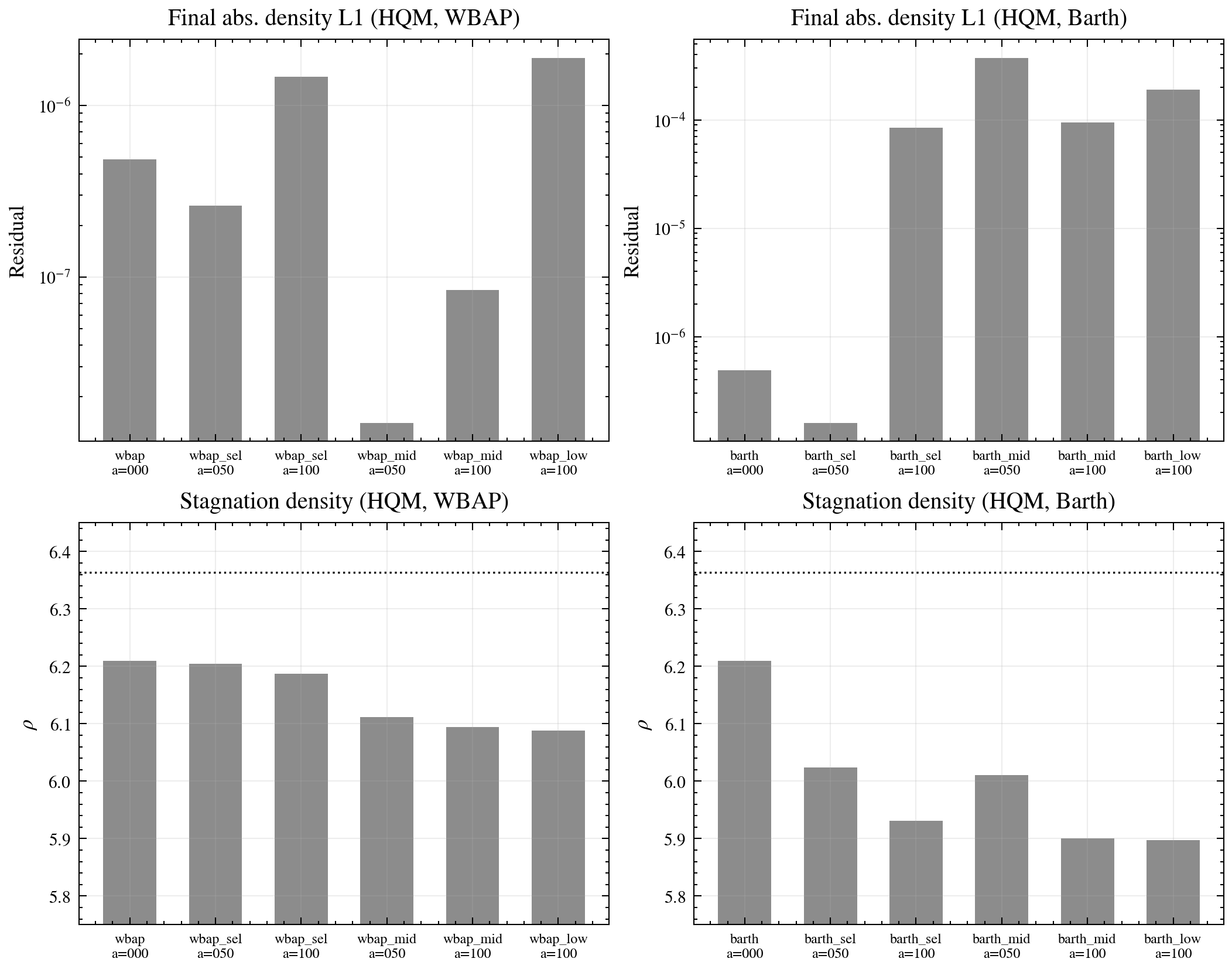
| Derivative-weight tuning | Compared Factorial and HQM_OPT reconstruction functionals; HQM_OPT reduced the Lax shoulder oscillation and improved the cylinder residual behavior. |
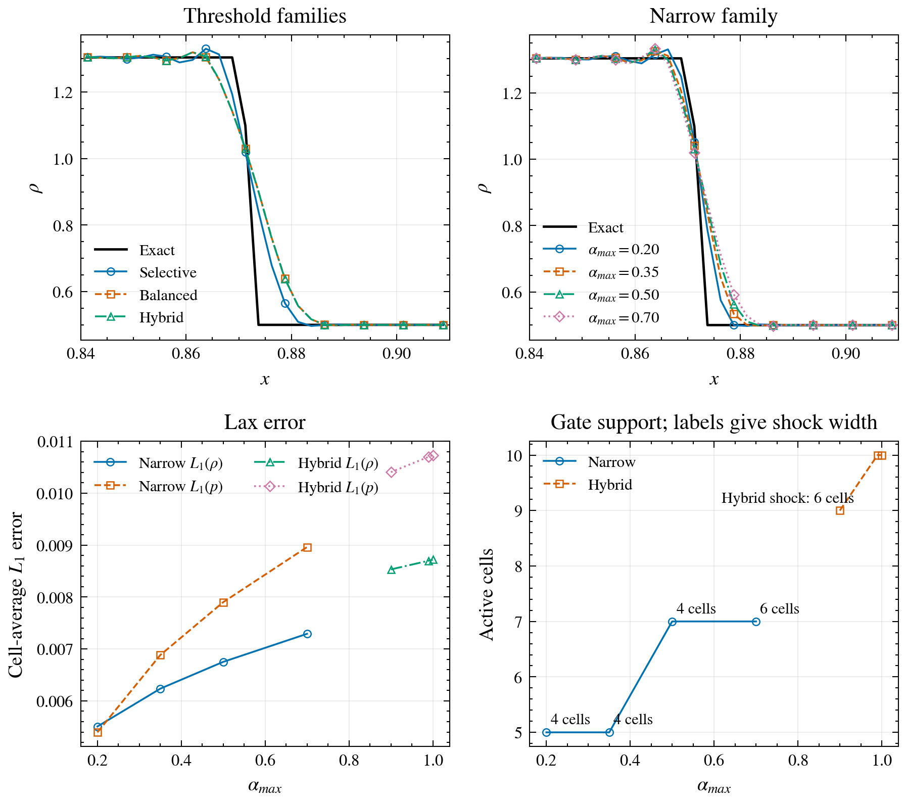
| Product-gate tuning | Tuned $j_{p0},j_{p1},j_{c0},j_{c1},\alpha_{max}$ on Lax and the Mach-20 cylinder, while retaining exactly zero penalty in smooth cells. |
| LVR v2 correction | Added the shock-supported extremum correction, retention, equal-neighbour guard, and bounded seed extension. |
| Flux and case extension | Tested Rusanov, Roe M8/M9, Sod, Toro 123, two-shock, Shu–Osher, and the cylinder. |
| Multidimensional production | Completed aligned and unstructured Double Mach reflection, the 13-method DM240U matrix, and both structured and matched-cell-count Delaunay 2-D Riemann comparisons. |
The detailed development reports are initial validation, parameter tuning, WBAP O2 retuning, HQM_OPT joint tuning, shock-band correction, and extended v2 validation. These links require access to the private study repository.
Lax shock-band reduction
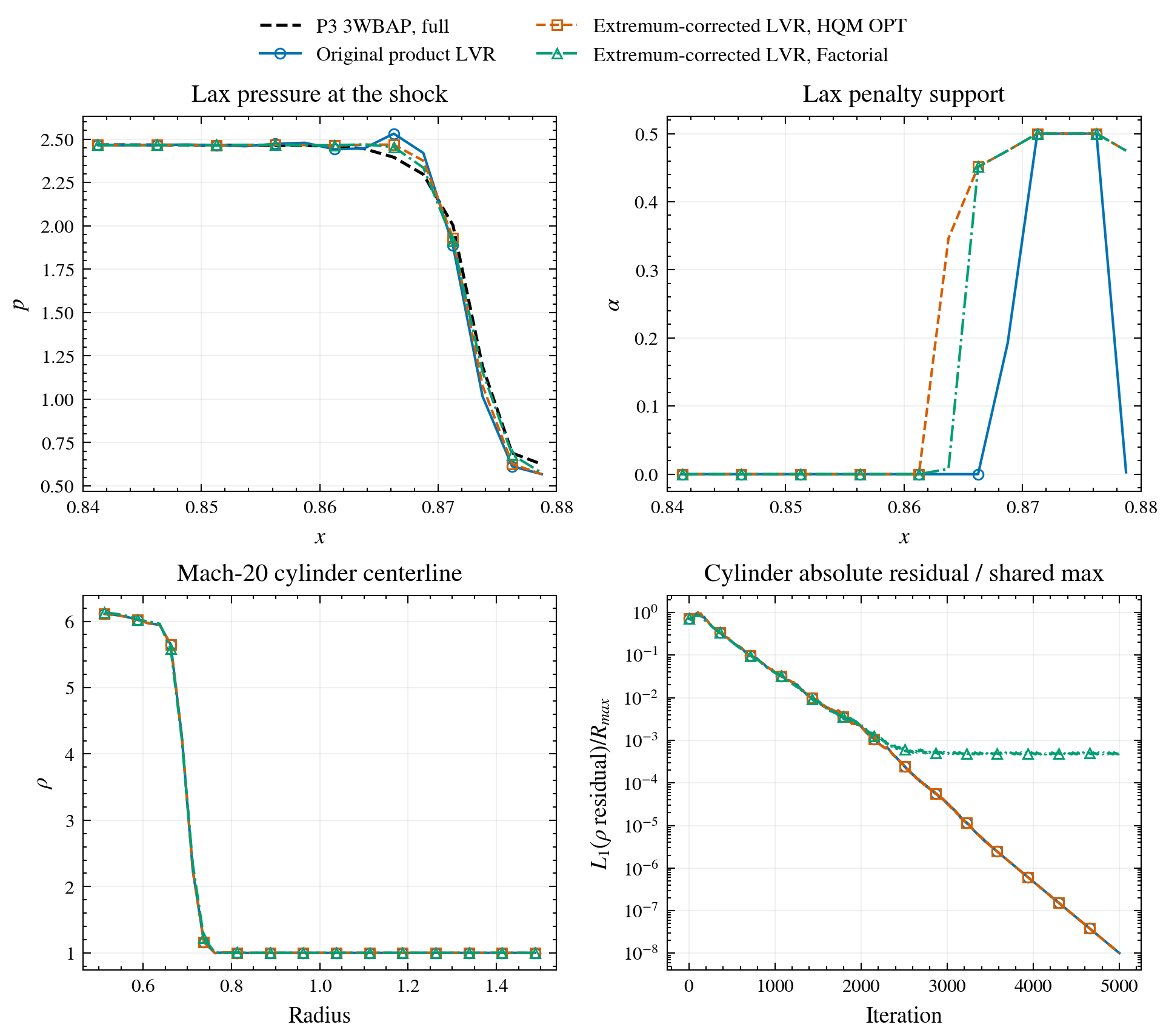
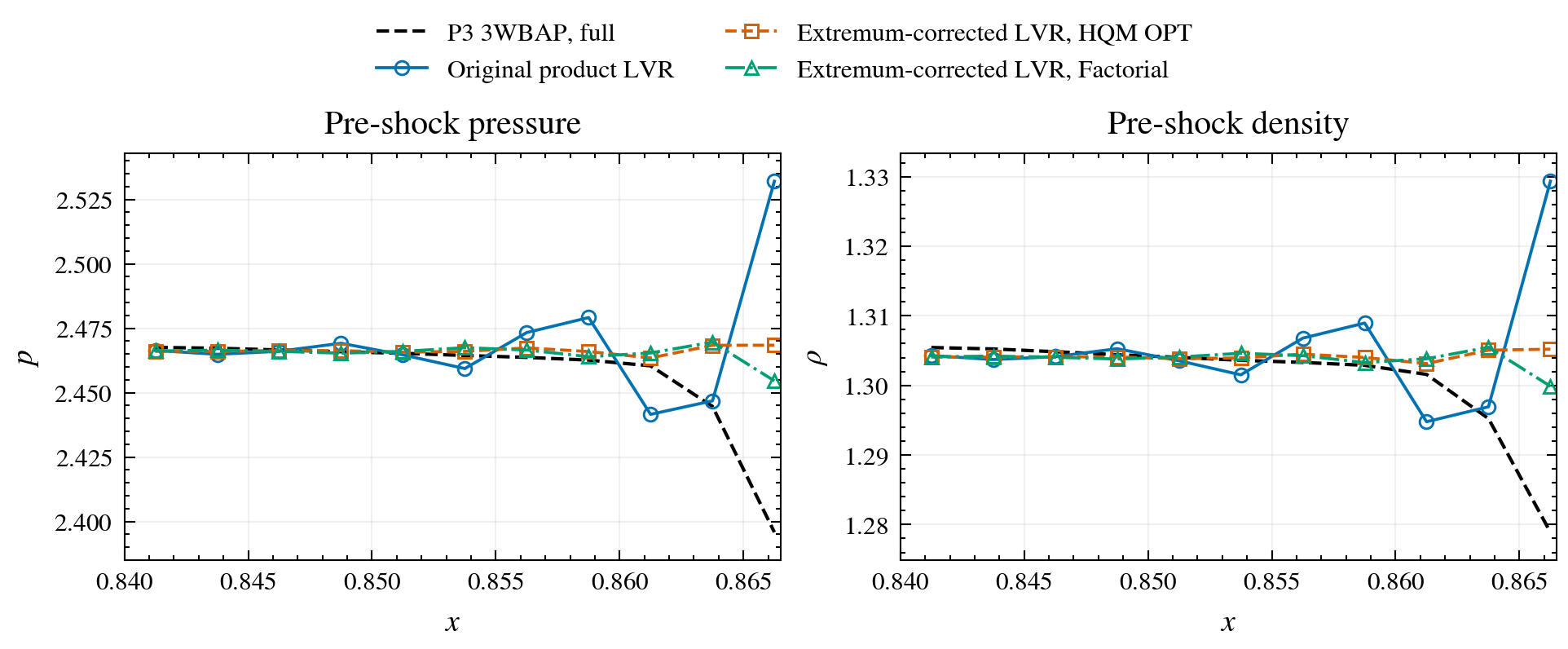
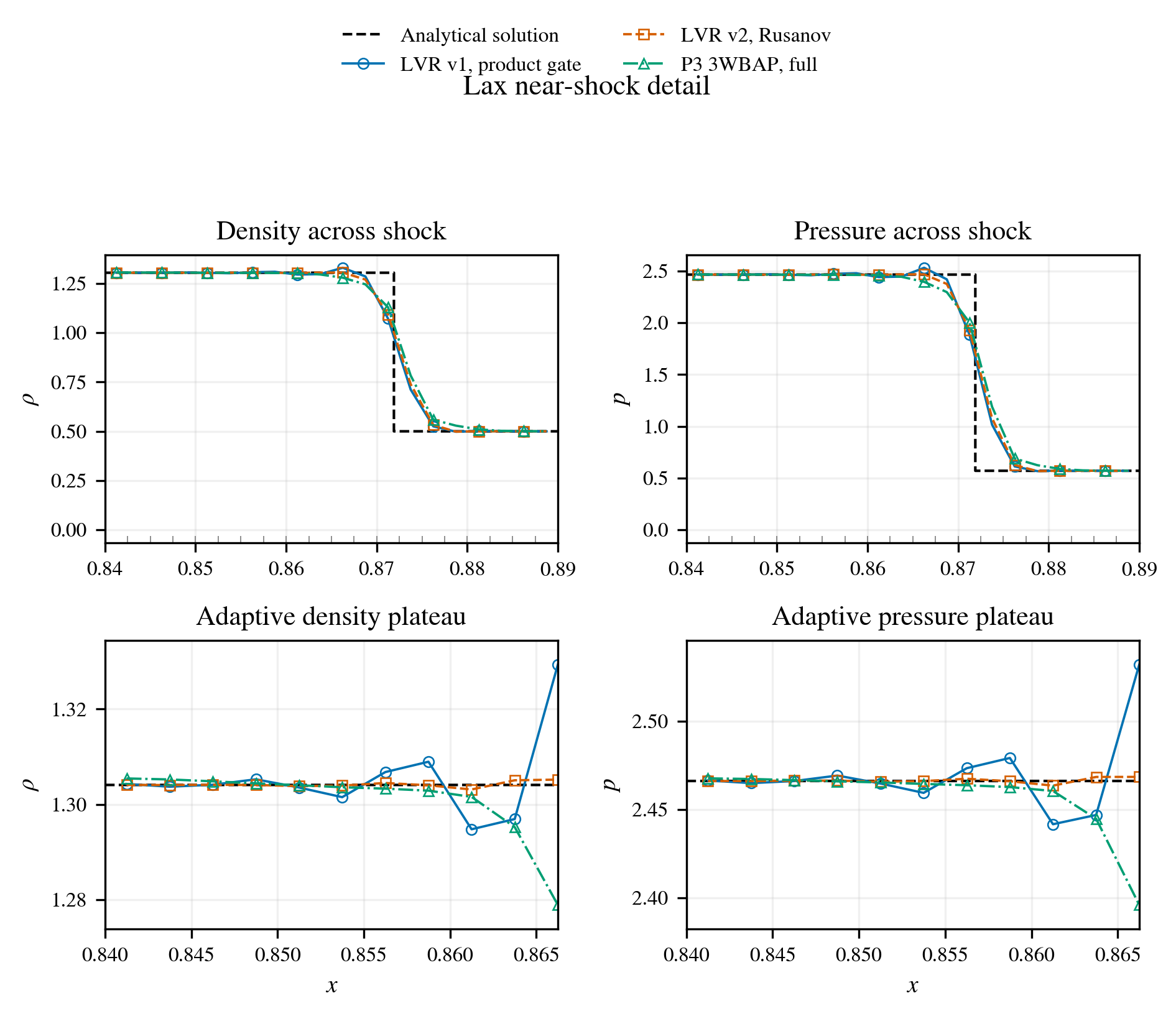
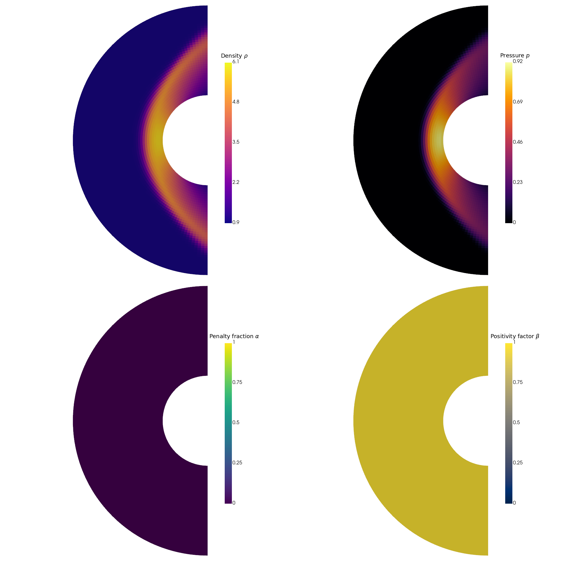
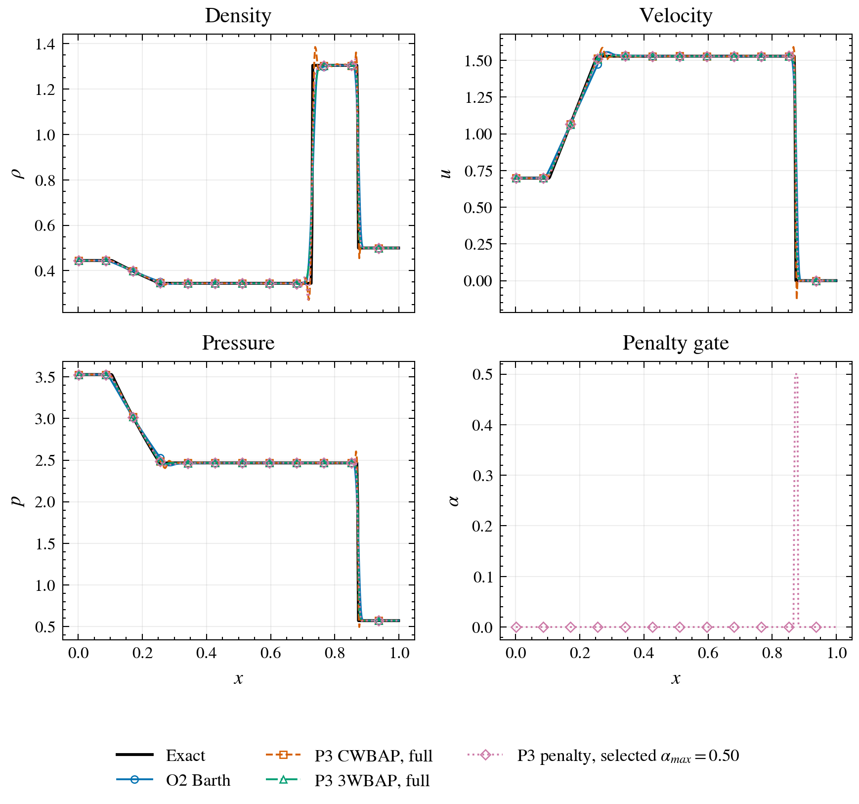
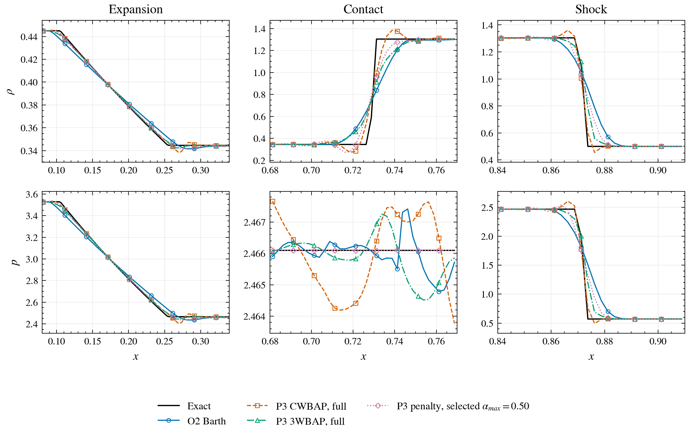
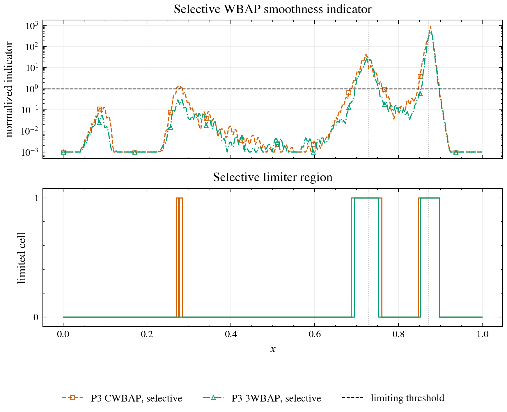
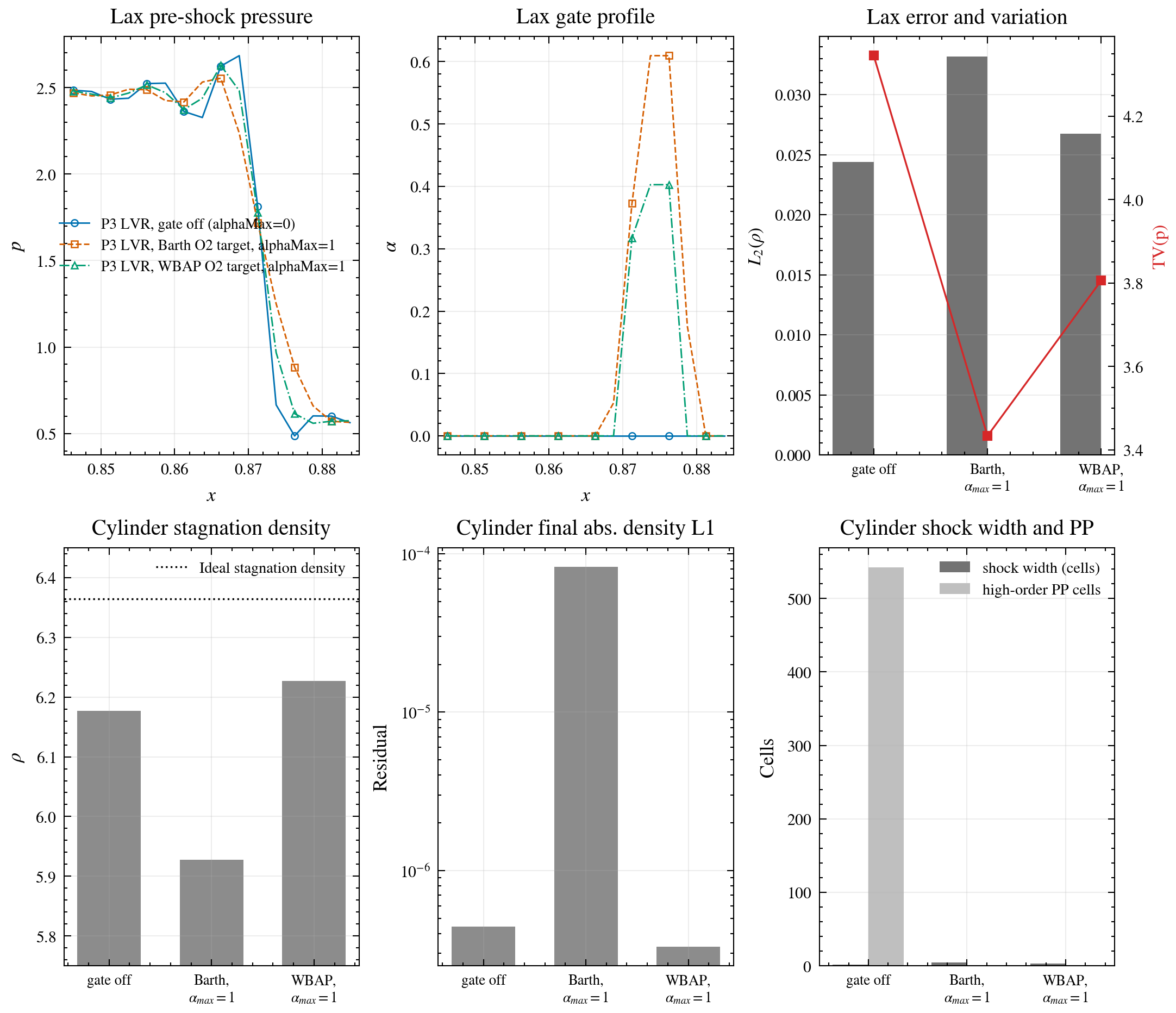
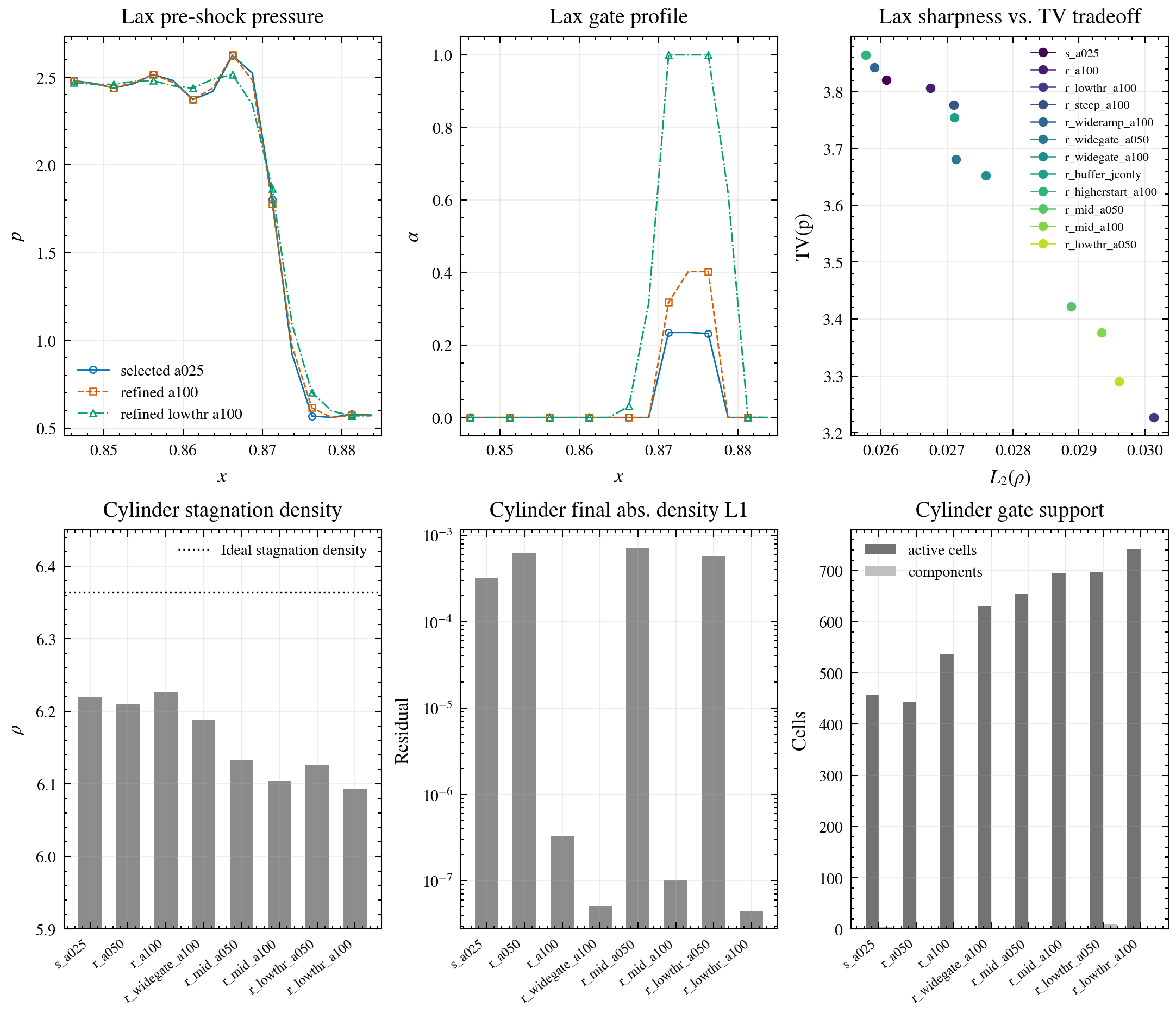
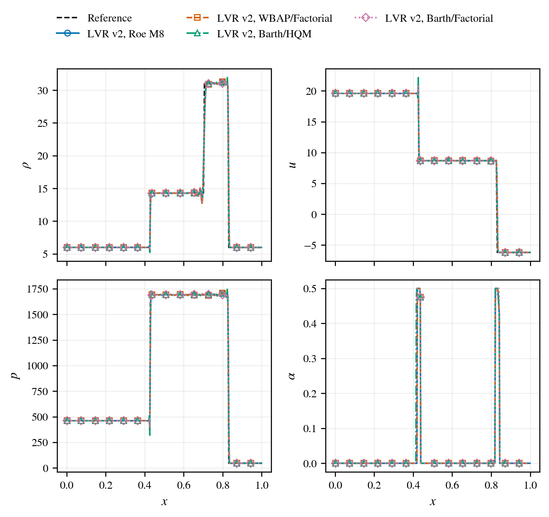
At $t=0.15$ on the maintained 400-cell Lax tube, the original product gate left a pressure overshoot/undershoot on the constant state immediately beside the right-moving shock. The corrected v2 gate expanded from five to nine active cells and nearly flattened this shoulder without changing the curved Mach-20 cylinder result.
| Method | Wrong-direction pressure excursion | Wrong-direction density excursion | Downstream left-plateau pressure range | Density $L_1$ | Active cells |
|---|---|---|---|---|---|
| Fully limited P3 3WBAP | 0 | 0 | 0.07173 | not reduced in this study | all |
| Original product LVR, WBAP O2, HQM_OPT | 0.11452 | 0.04356 | 0.09046 | $4.208\times10^{-3}$ | 5 |
| LVR v2, WBAP O2, HQM_OPT | 0.00686 | 0.00279 | 0.00495 | $4.284\times10^{-3}$ | 9 |
| LVR v2, WBAP O2, Factorial | 0.00808 | 0.00313 | 0.01502 | $5.725\times10^{-3}$ | 9 |
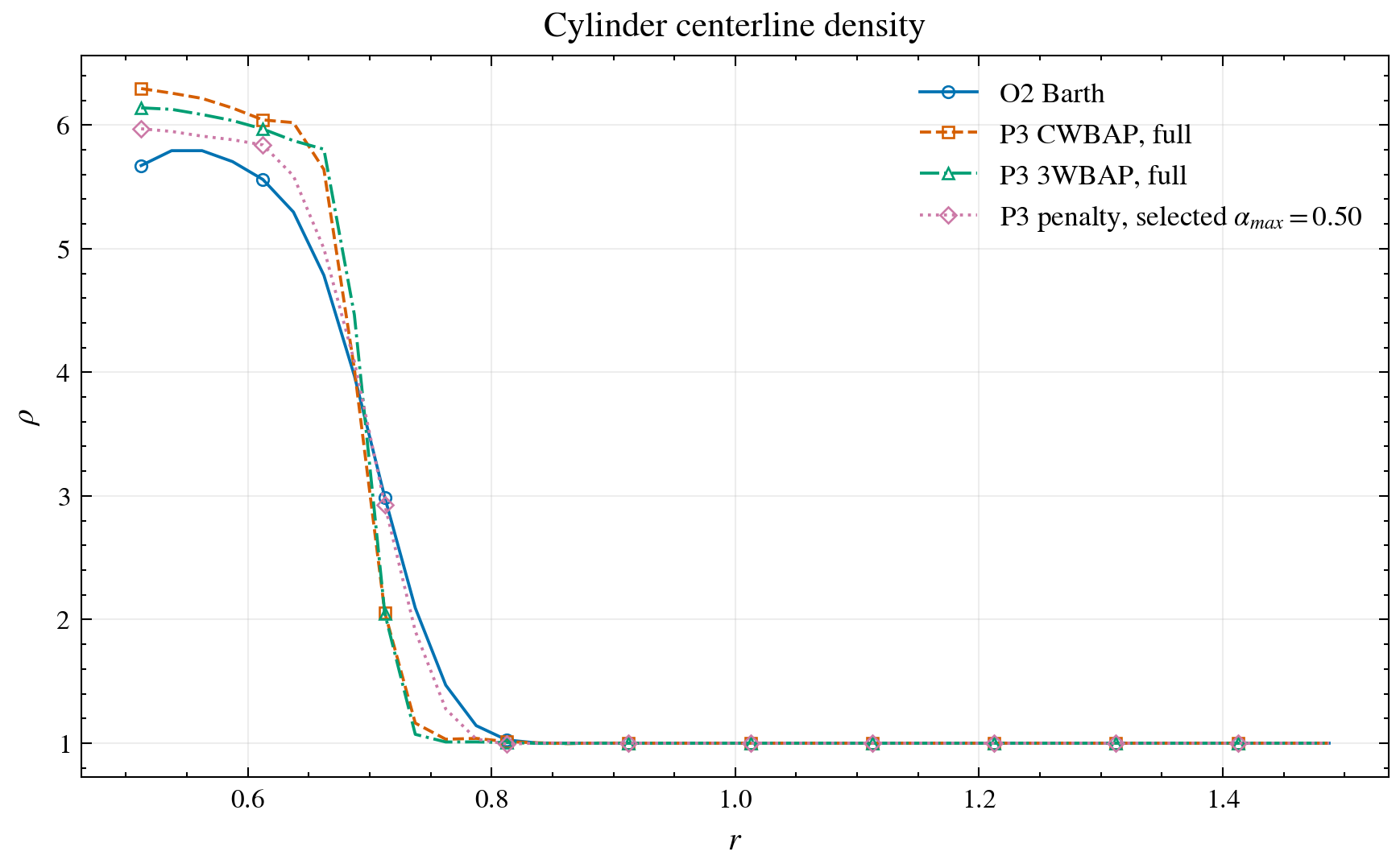
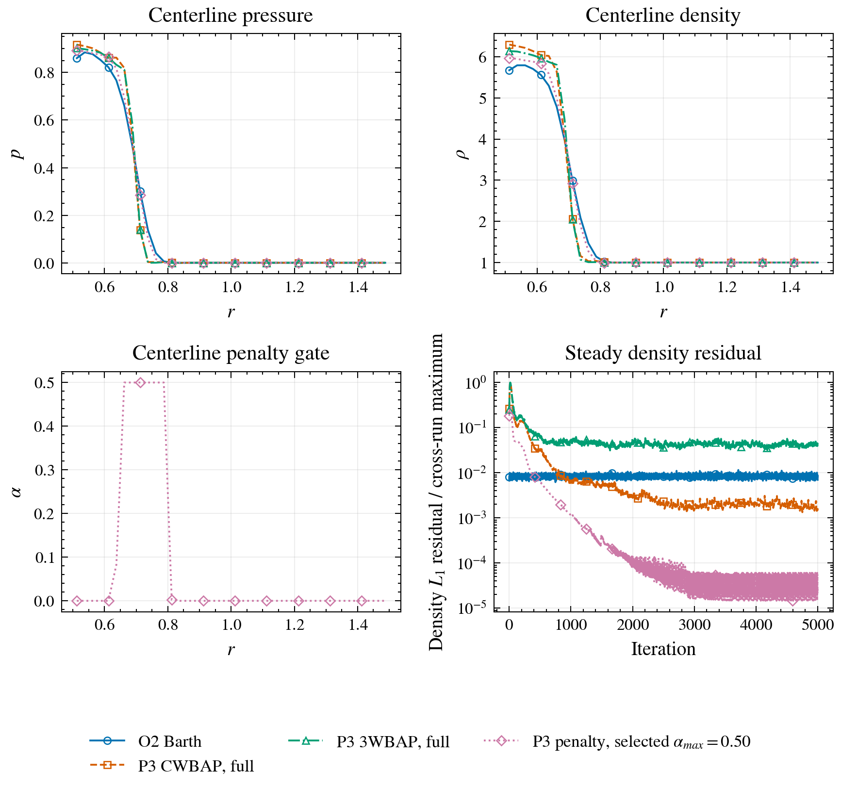
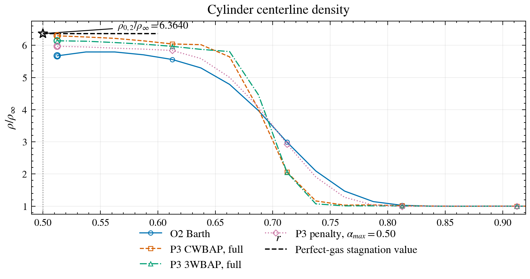
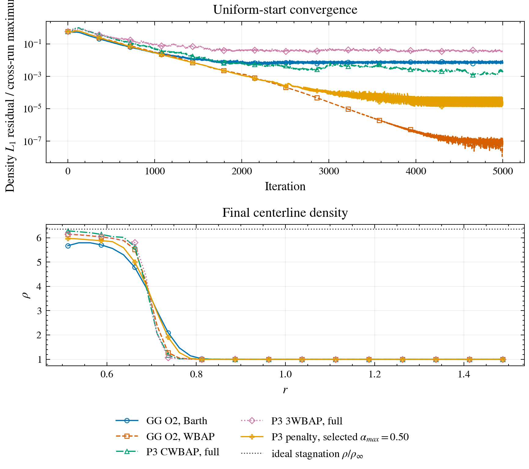
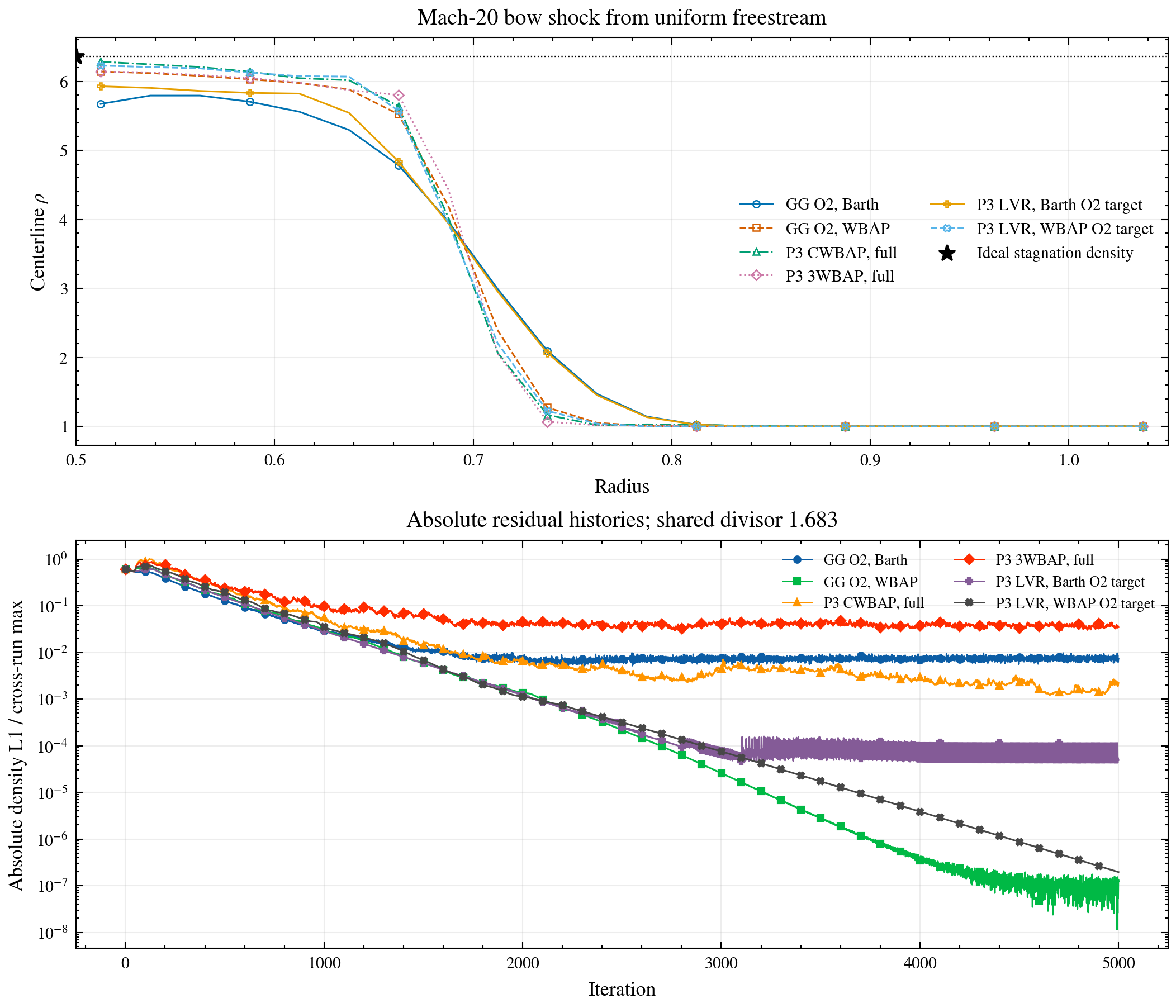
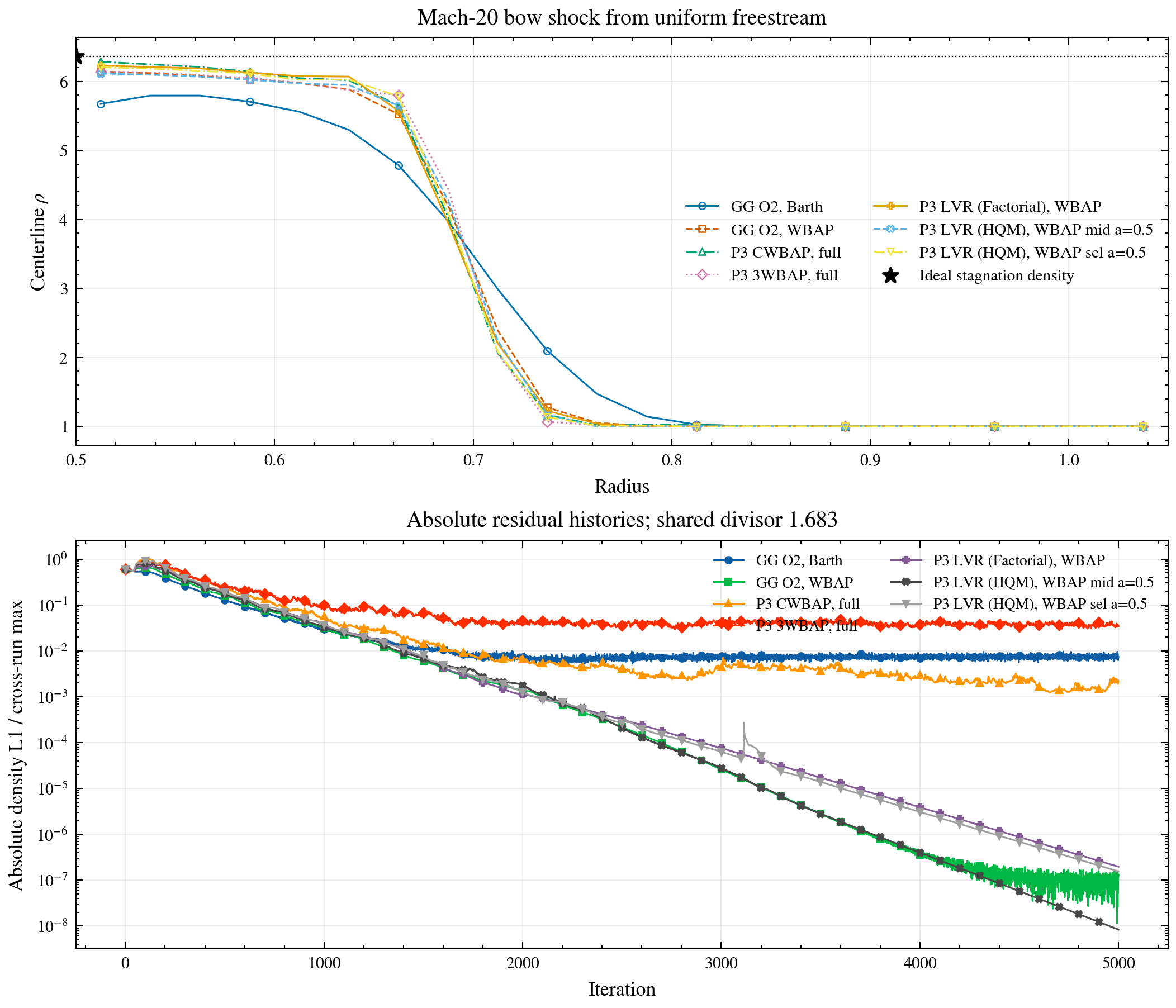
For this right-moving shock, the nearly constant region immediately to its left is the downstream, post-shock plateau. For HQM_OPT, the correction reduces the pressure excursion by 94.0% and that plateau’s pressure range by 94.5%, while density $L_1$ rises only 1.8%. On the Mach-20 cylinder, corrected and original HQM_OPT histories are numerically identical: final absolute density $L_1$ residual $1.405\times10^{-8}$, 684 active cells, no wall or far-field activation, a two-cell centerline shock, and stagnation density 6.11134.
Extended compact-case validation
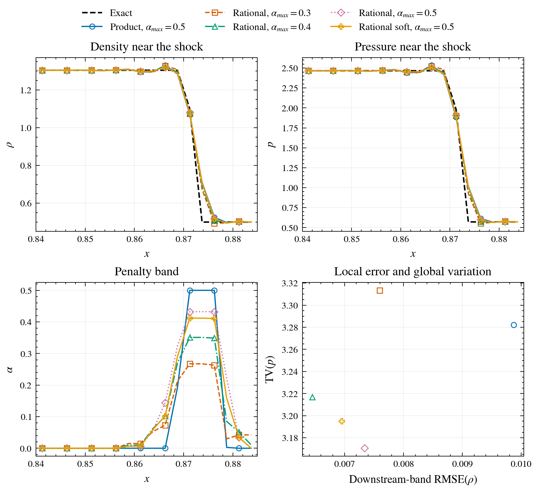
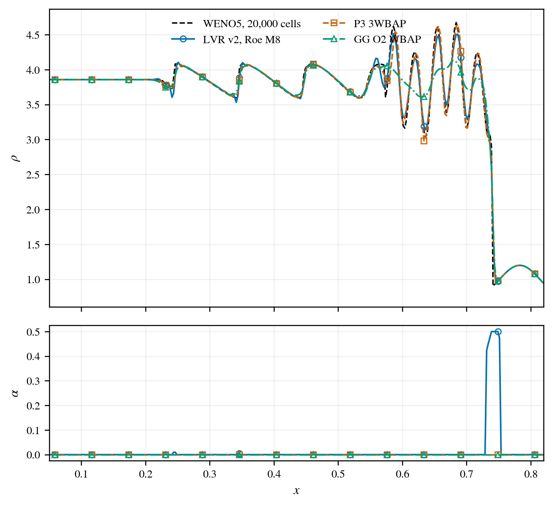
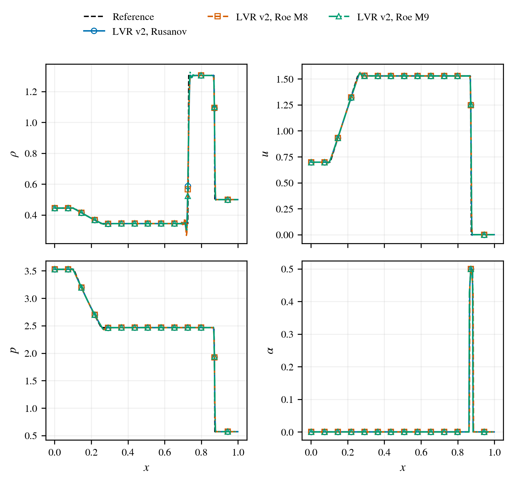
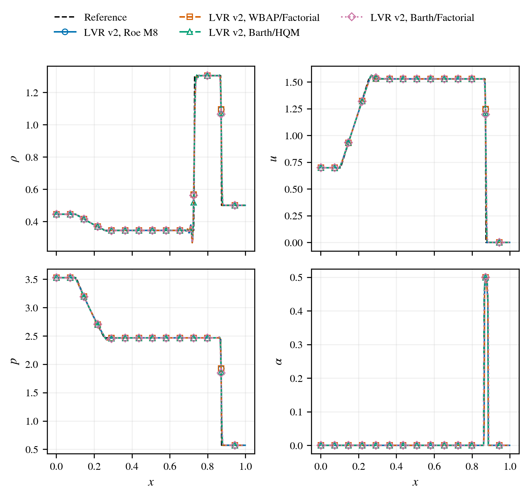
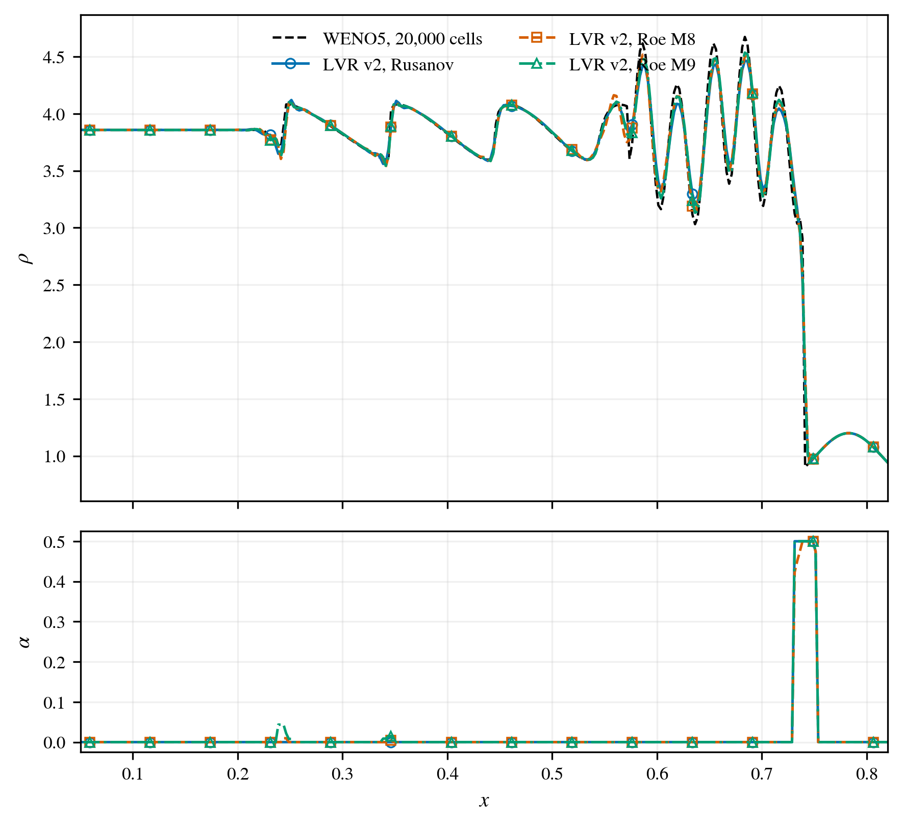
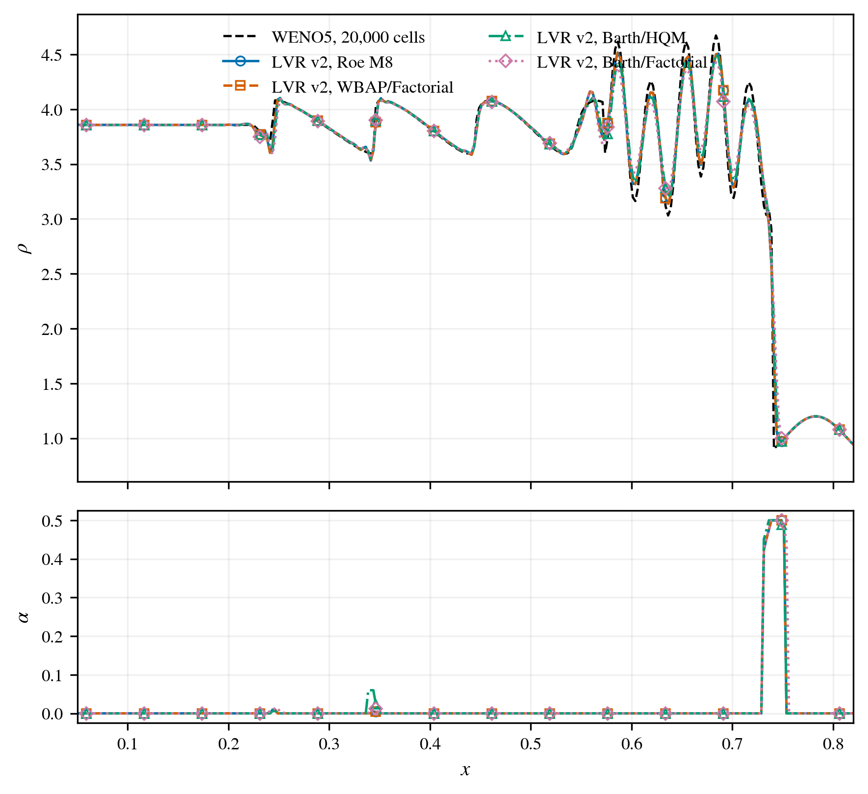
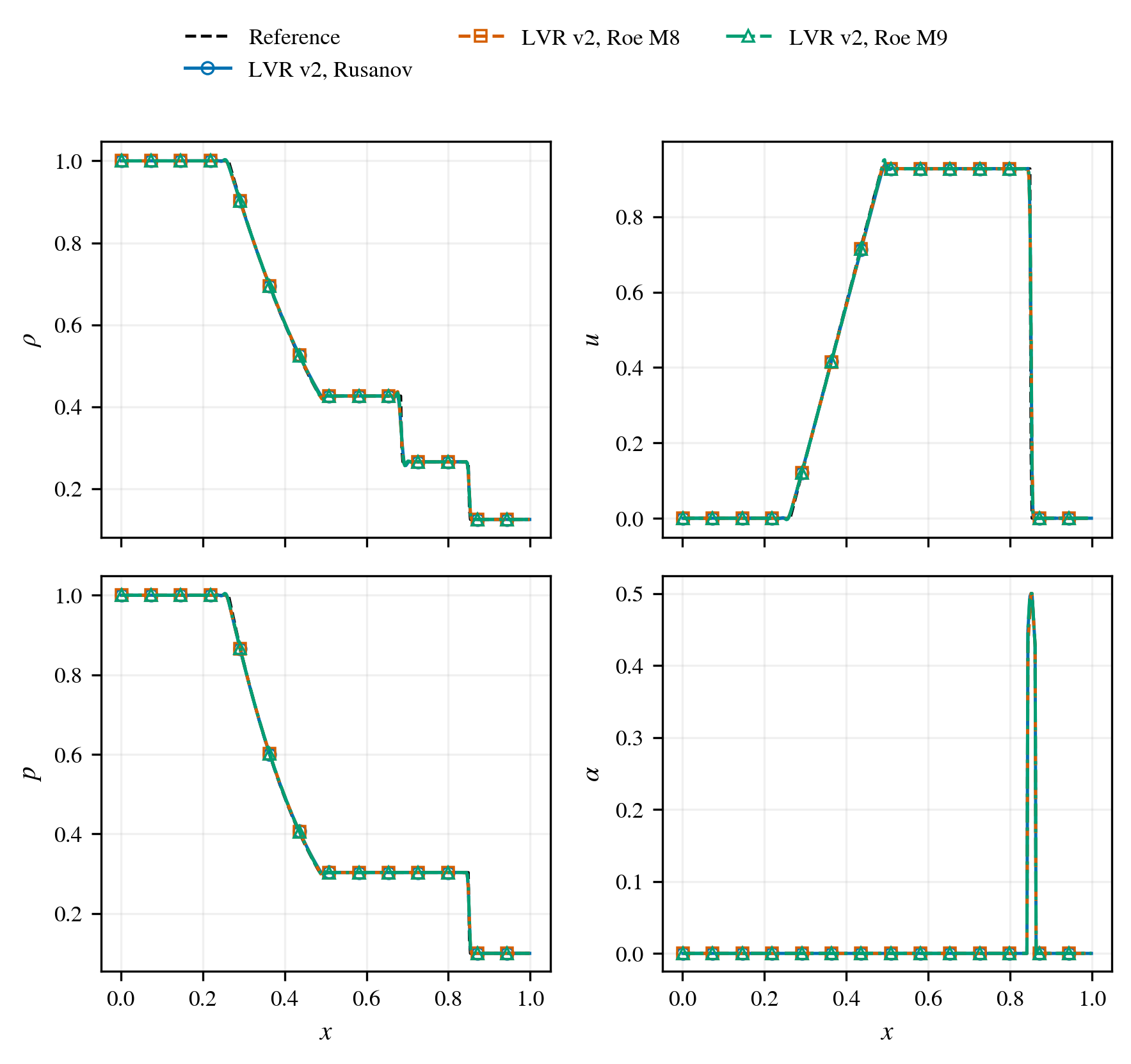
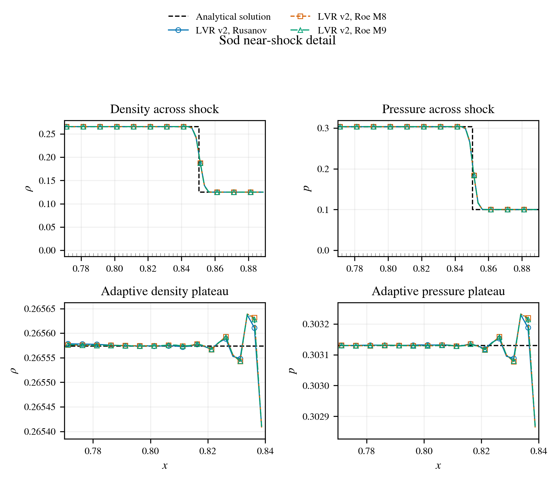
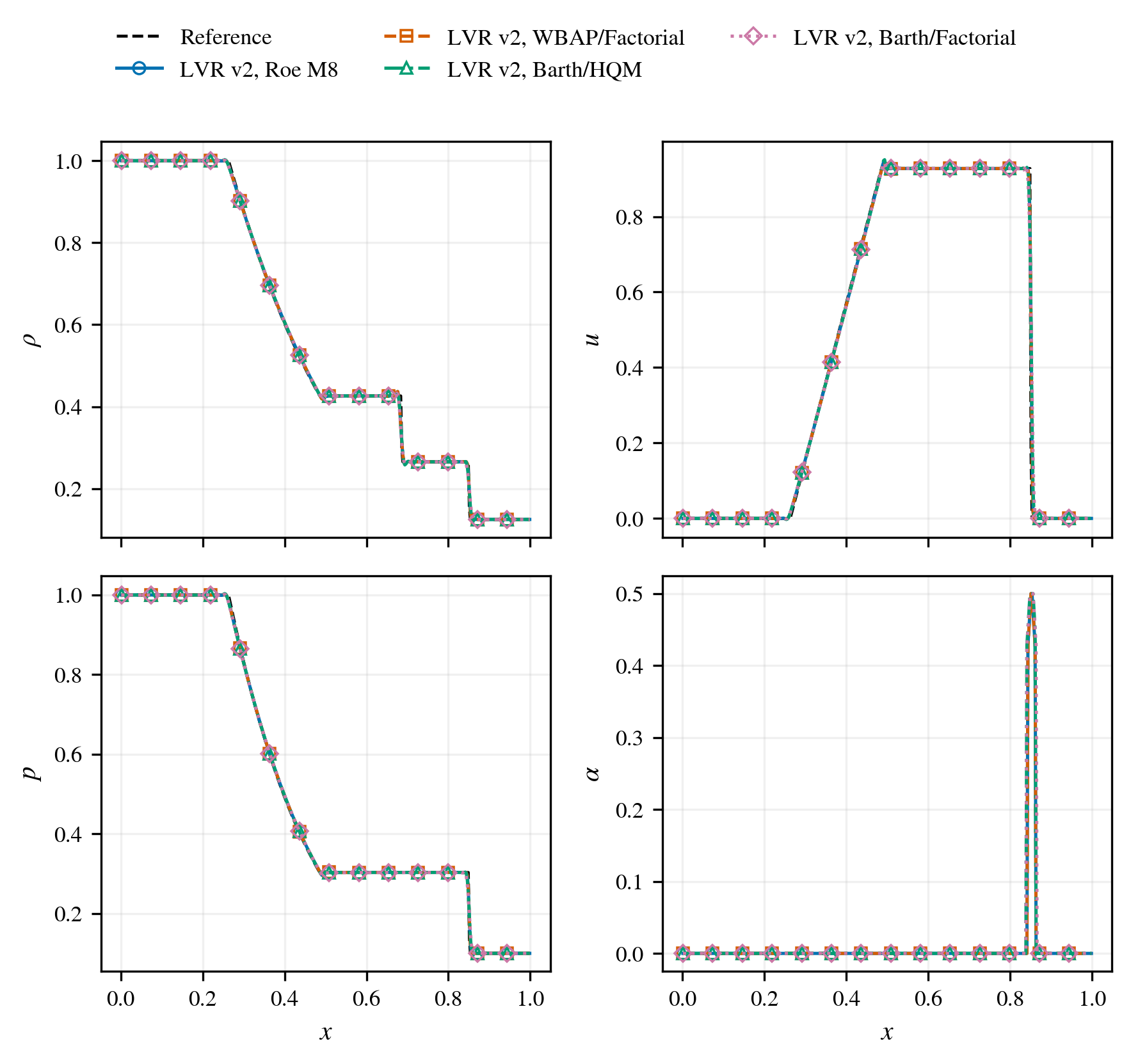
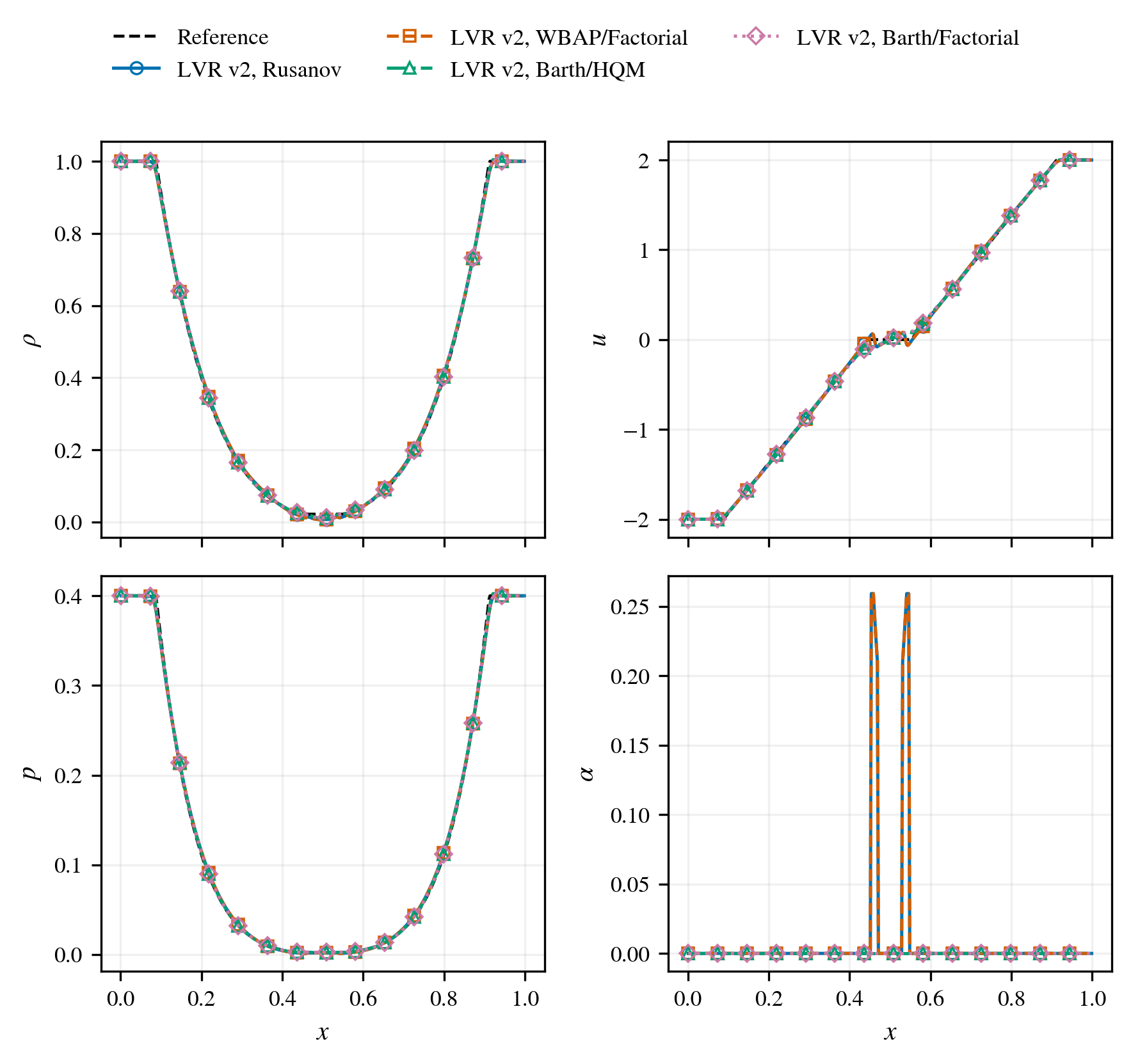
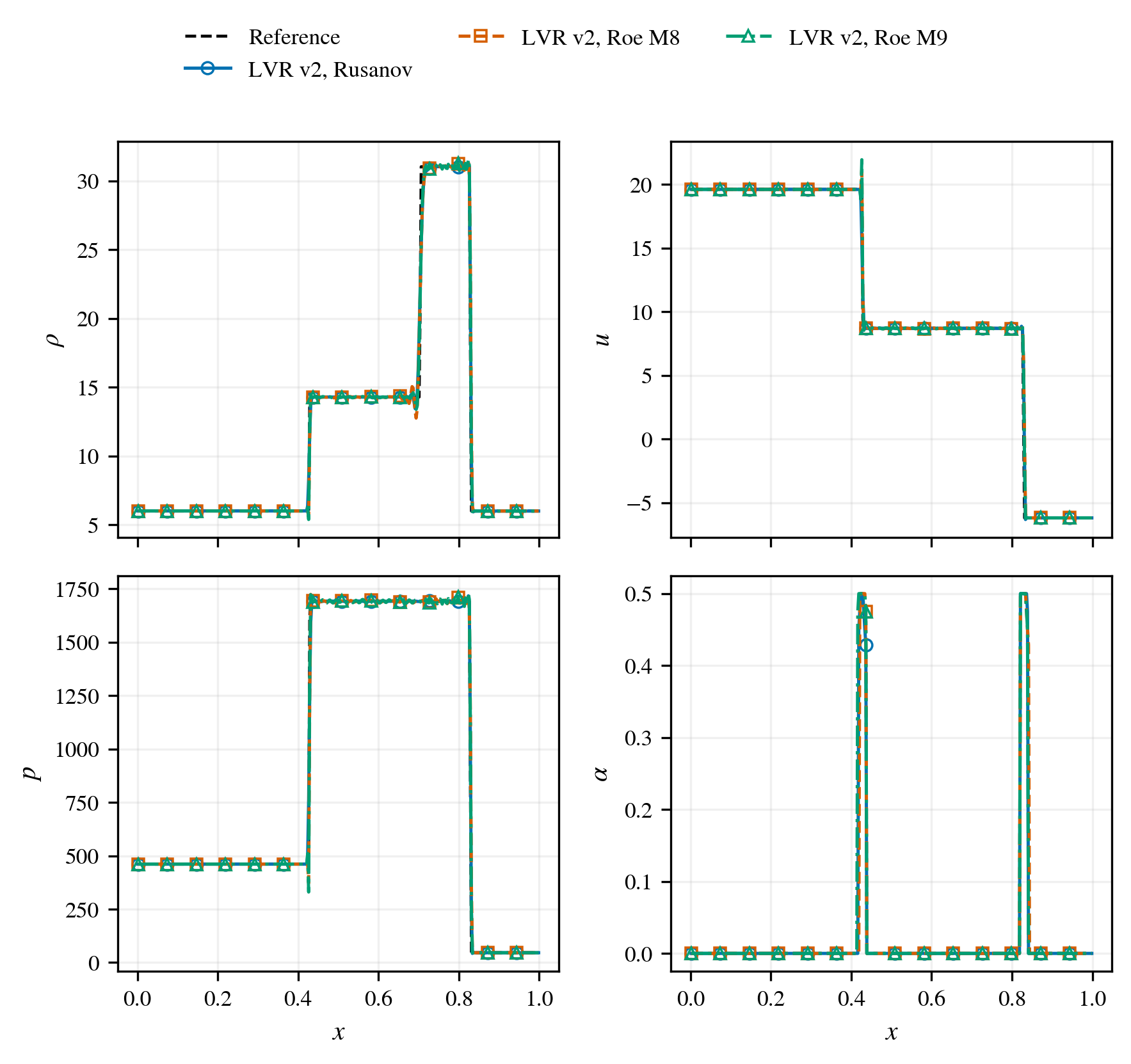
The extended study used exact cell-averaged Riemann solutions and an independent 20,000-cell characteristic WENO5 reference for Shu–Osher. Roe M8 and M9 reduce Lax, Sod, two-shock, and Shu–Osher errors relative to Rusanov, but both Roe variants stall on the Toro 123 double-rarefaction case with the tested positivity configuration. Rusanov remains the robust cylinder choice.
Representative density $L_1$ values for LVR v2/HQM_OPT are:
| Case | Rusanov | Roe M8 | Roe M9 |
|---|---|---|---|
| Lax | 0.004310 | 0.003594 | 0.003602 |
| Sod | 0.001491 | 0.001282 | 0.001285 |
| Toro 123 double rarefaction | 0.004974 | stalled | stalled |
| Two-shock | 0.09827 | 0.09648 | 0.09630 |
| Shu–Osher | 0.03055 | 0.02341 | 0.02359 |
The v2 correction is intentionally narrow: it fixes the Lax weak-gate gap, remains inactive on the curved cylinder bow shock, and does not turn the whole post-shock Shu–Osher wave train into an O2 solution.
Canonical 13-method matrix
The thtj1 campaign compares 13 configurations:
- Explicit GG O2 with WBAP limiting;
- LVR v2 with WBAP O2 target, HQM_OPT weights, $\alpha_{max}=0.5$;
- the same with $\alpha_{max}=1$;
- LVR v2 with WBAP O2 target, Factorial weights, $\alpha_{max}=0.5$;
- the same with $\alpha_{max}=1$;
- LVR v2 with Barth O2 target, HQM_OPT weights, $\alpha_{max}=0.5$;
- the same with $\alpha_{max}=1$;
- LVR v2 with Barth O2 target, Factorial weights, $\alpha_{max}=0.5$;
- the same with $\alpha_{max}=1$;
- fully limited P3 3WBAP with HQM_OPT weights;
- fully limited P3 3WBAP with Factorial weights;
- fully limited P3 CWBAP with HQM_OPT weights;
- fully limited P3 CWBAP with Factorial weights.
The compact suite contains the Mach-20 cylinder plus Lax, Sod, Toro 123, two-shock, and Shu–Osher: 78 runs in total. Every run completed. The two tables below present every case twice. The first layout overlays all 13 methods in one plot. The second uses a controlled $2\times2$ layout to isolate method family, derivative weights, $\alpha_{max}$, and O2-target limiter.
All 13 methods in one layout
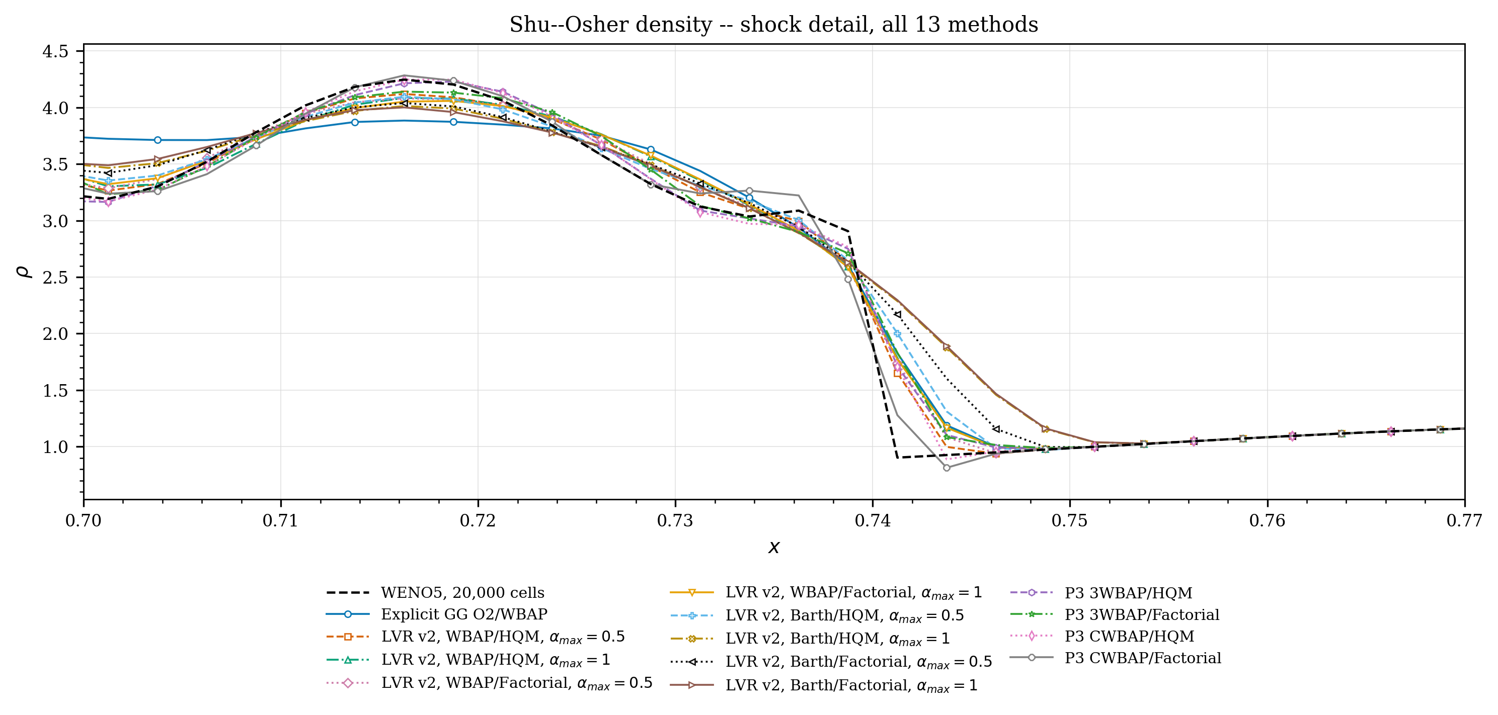
Each row gives the full case and a detailed view. Shock-tube details include states on both sides of the selected wave. Toro 123 has no shock, so its detail crosses the right rarefaction front. The Shu–Osher detail focuses on the post-shock entropy-wave train. For the steady cylinder, the complementary detail is the absolute density $L_1$ residual history because it distinguishes convergence floors that are hidden by the final centerline profile.
| Case | Full view, all 13 methods | Detailed view, all 13 methods |
|---|---|---|
| Mach-20 cylinder | 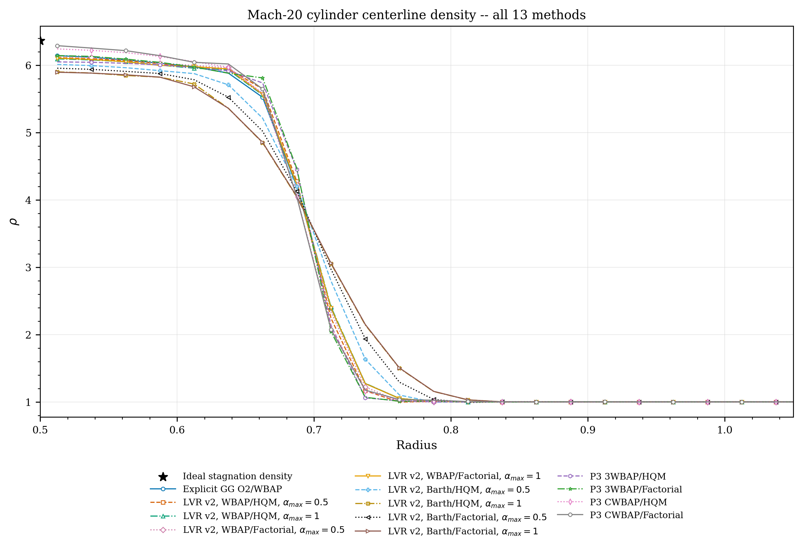 | 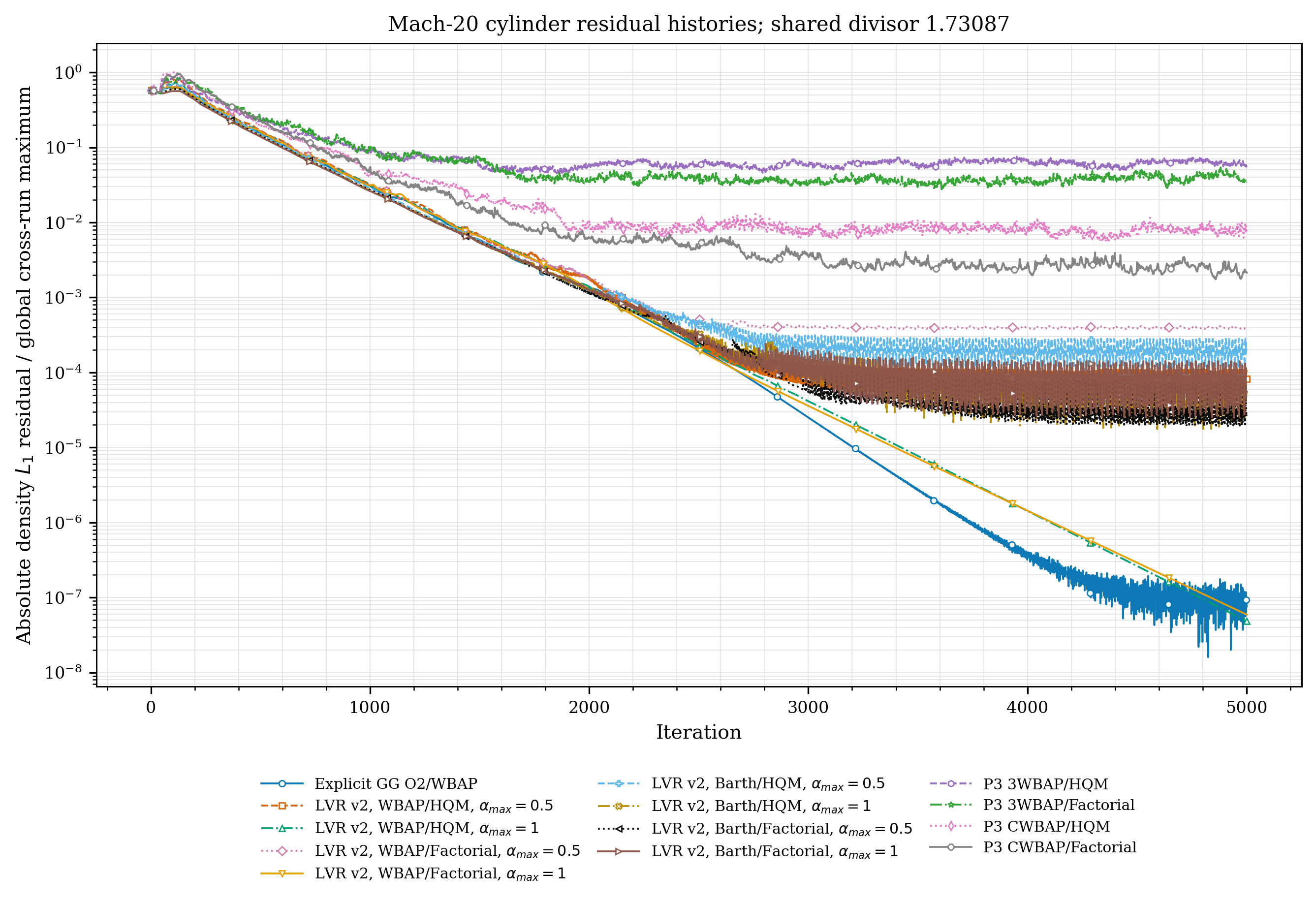 |
| Lax shock tube | 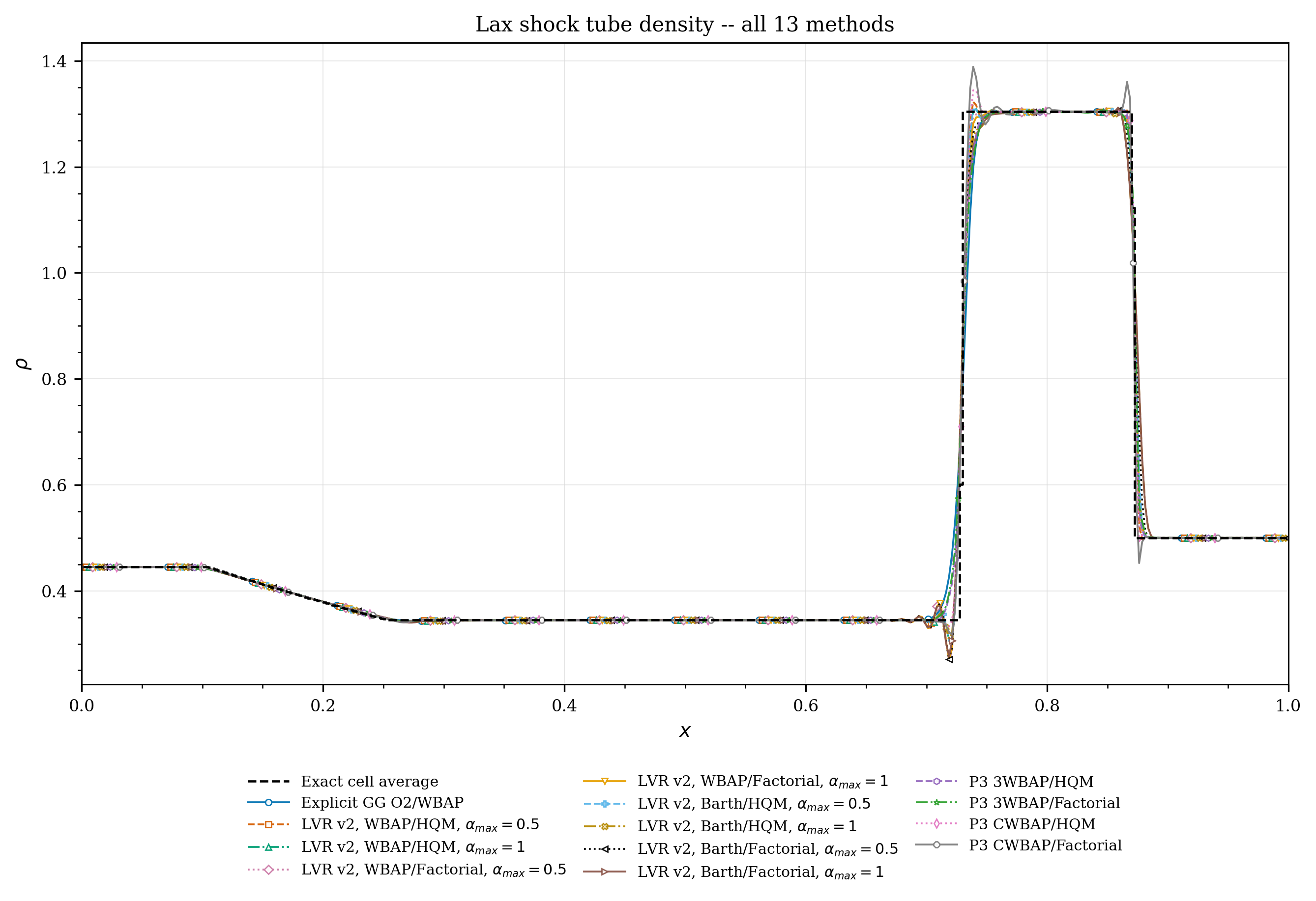 | 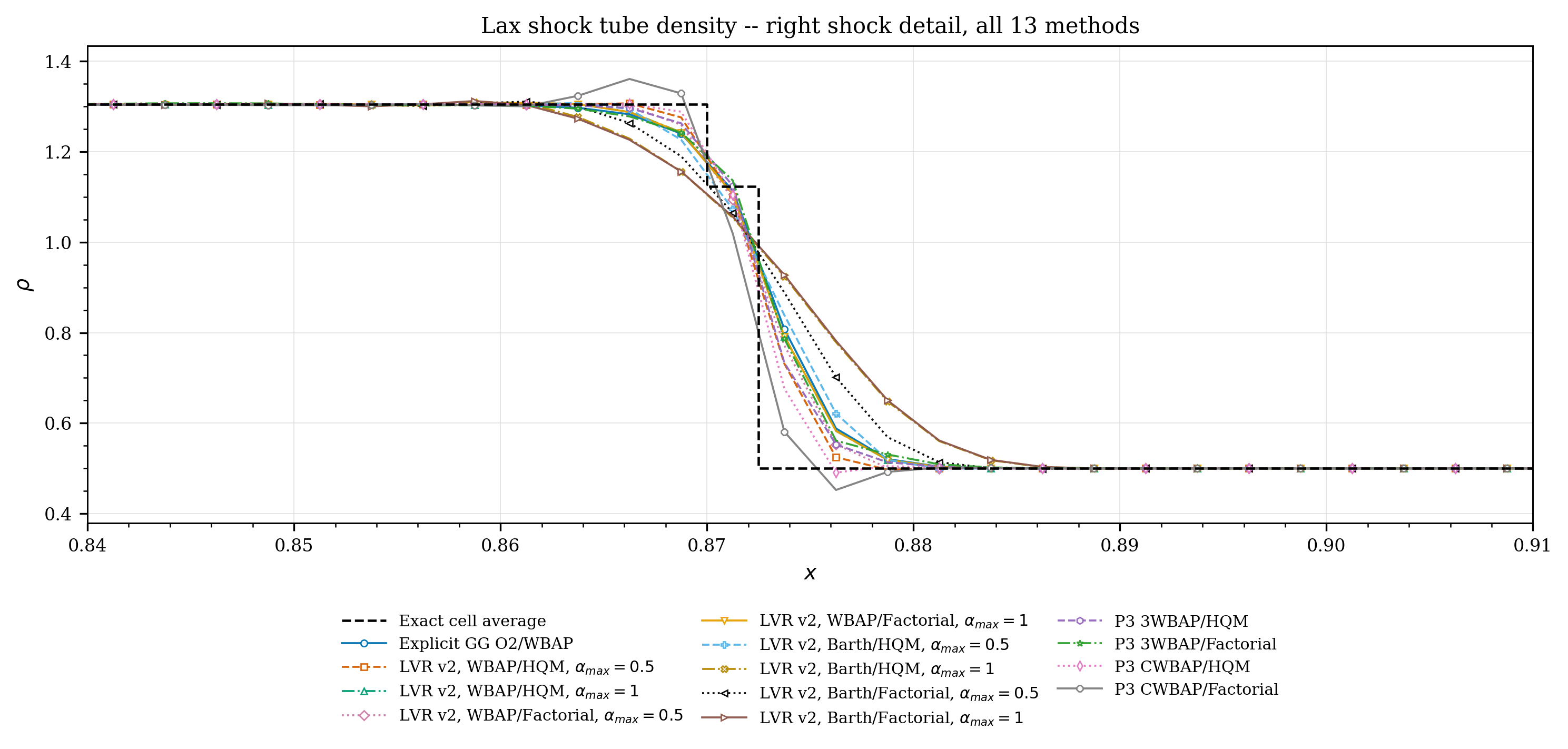 |
| Sod shock tube | 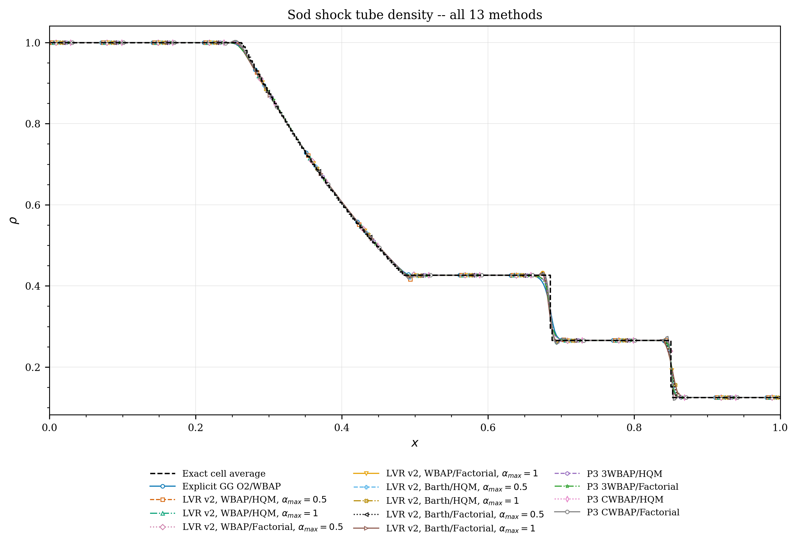 | 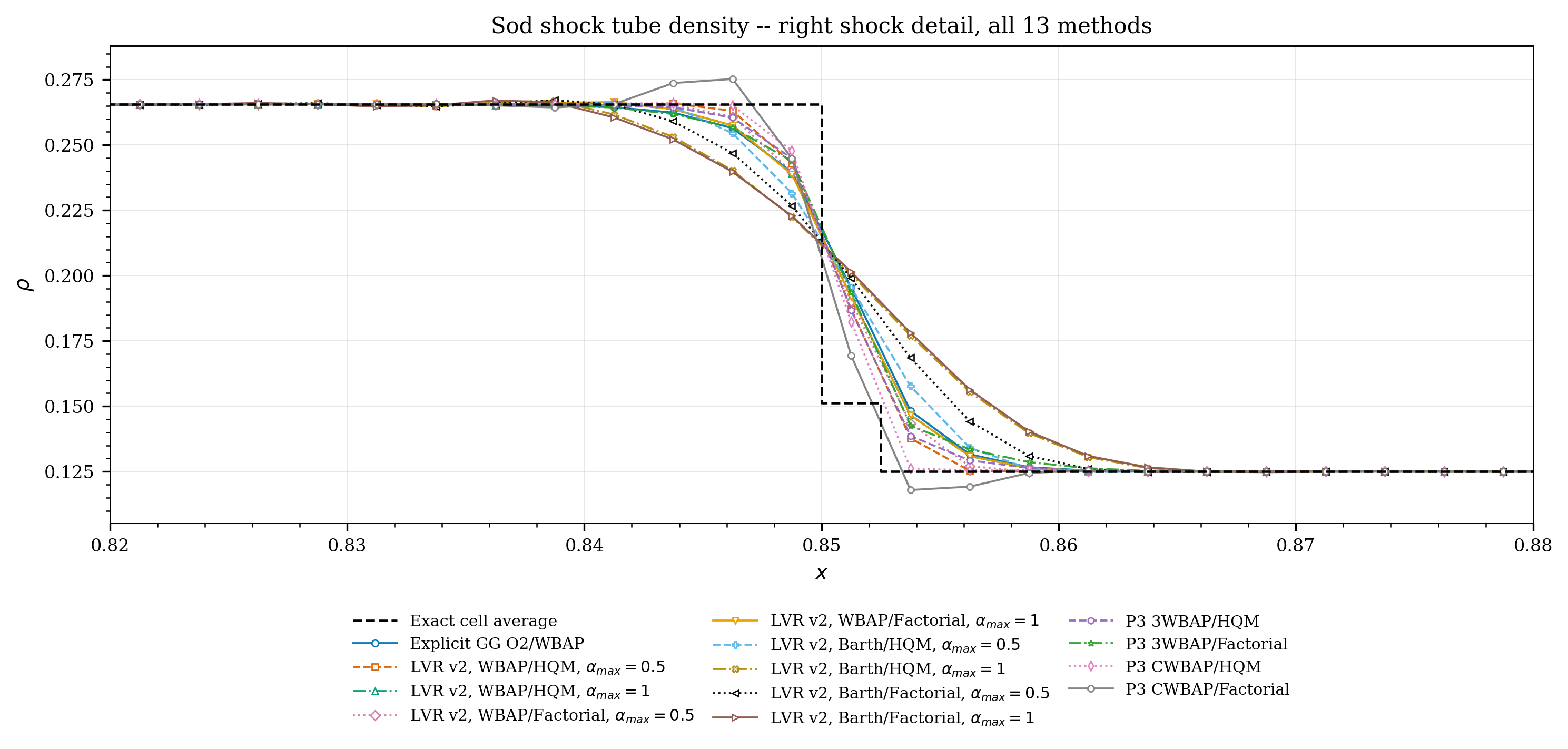 |
| Toro 123 double rarefaction | 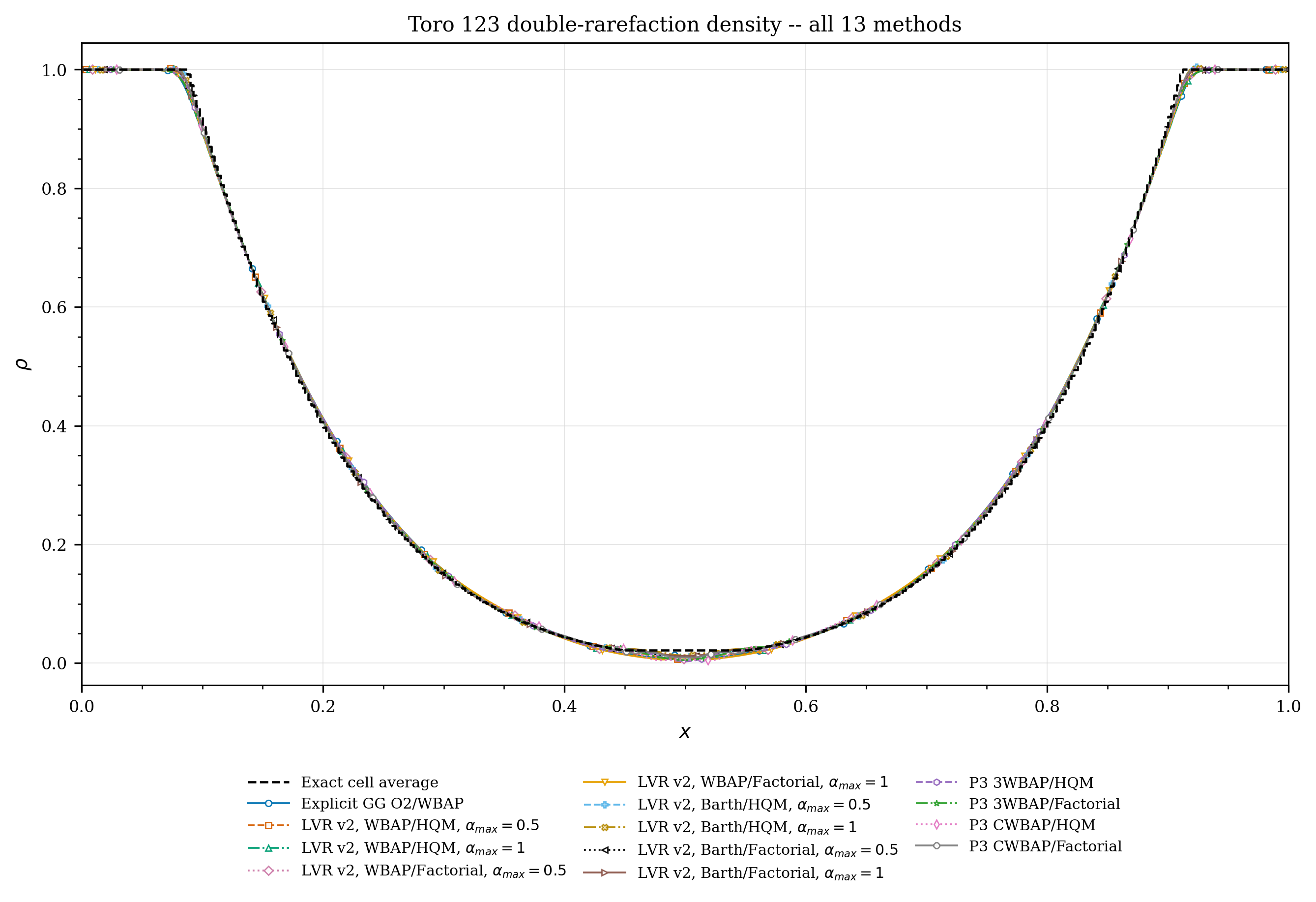 | 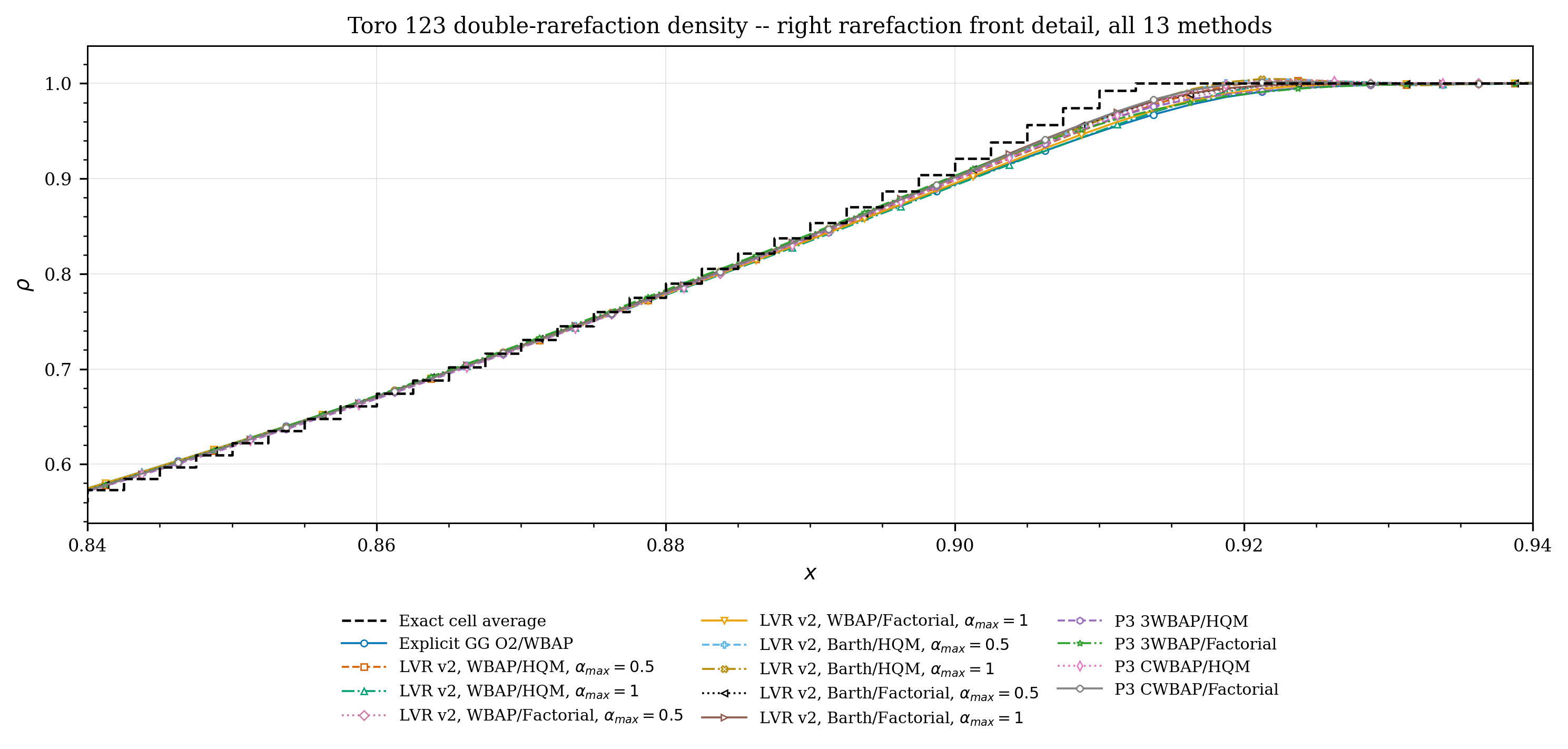 |
| Two-shock problem | 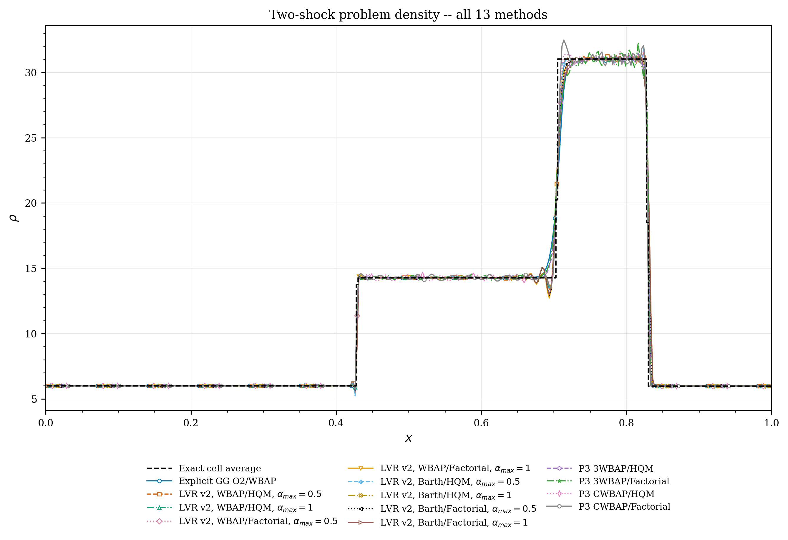 | 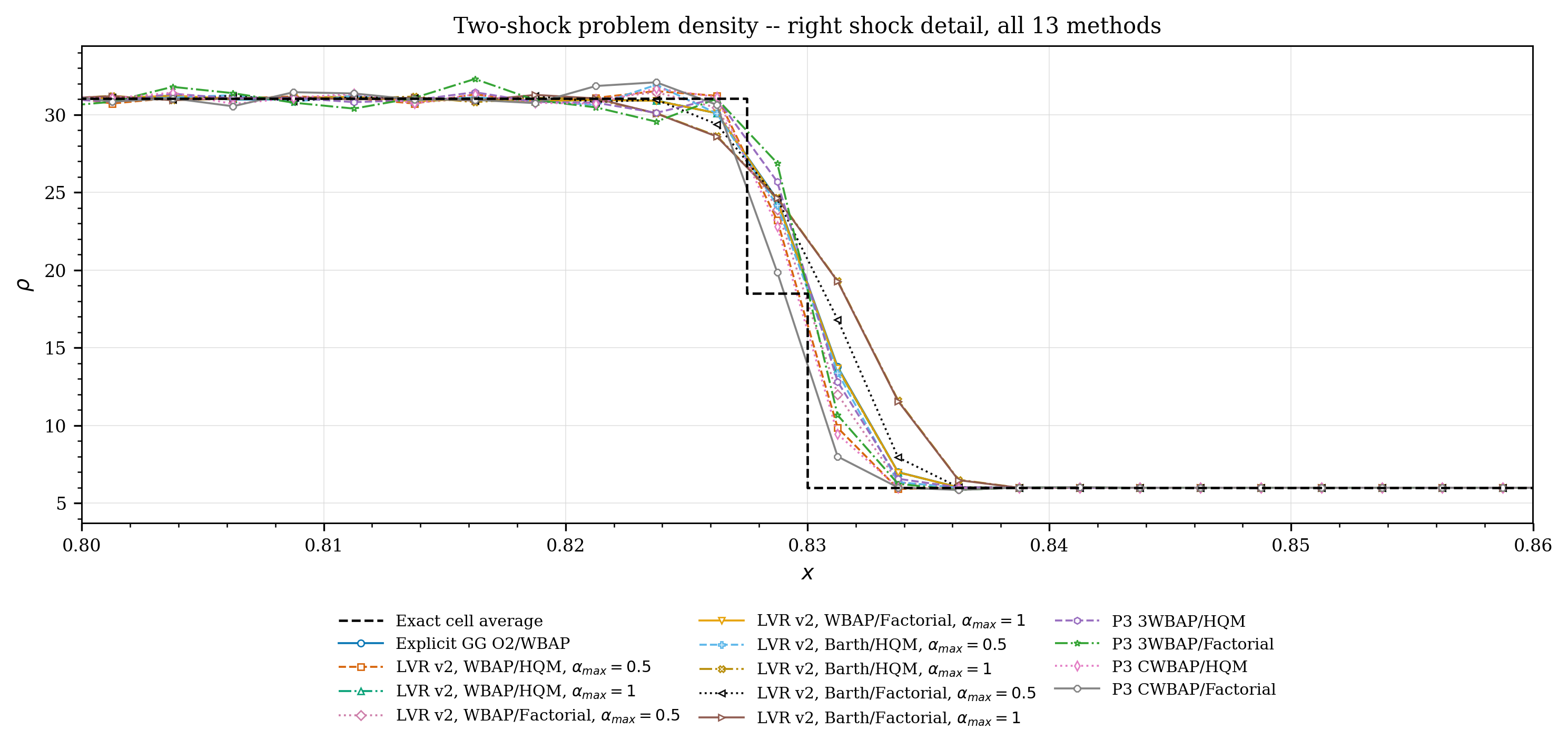 |
| Shu–Osher | 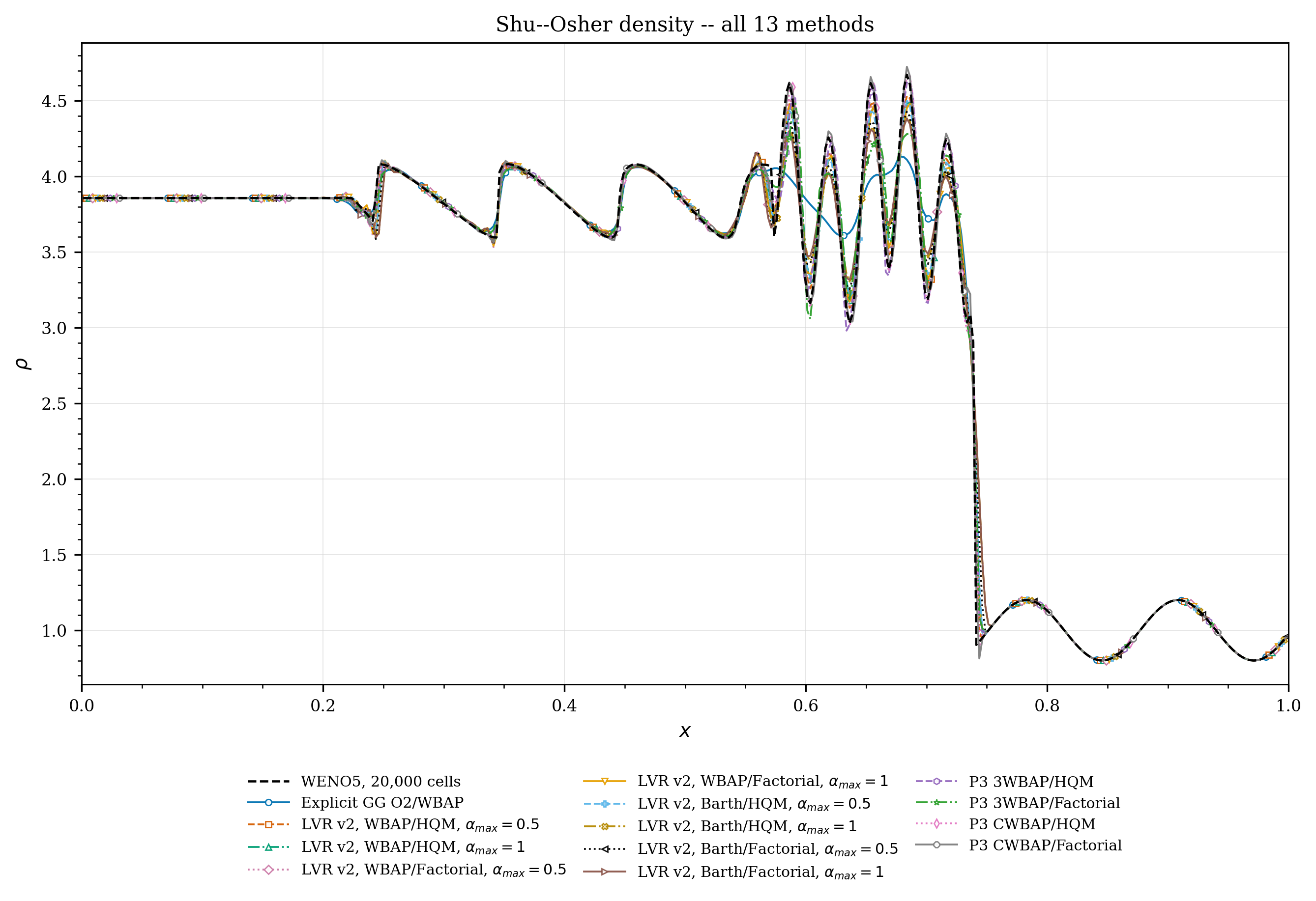 | 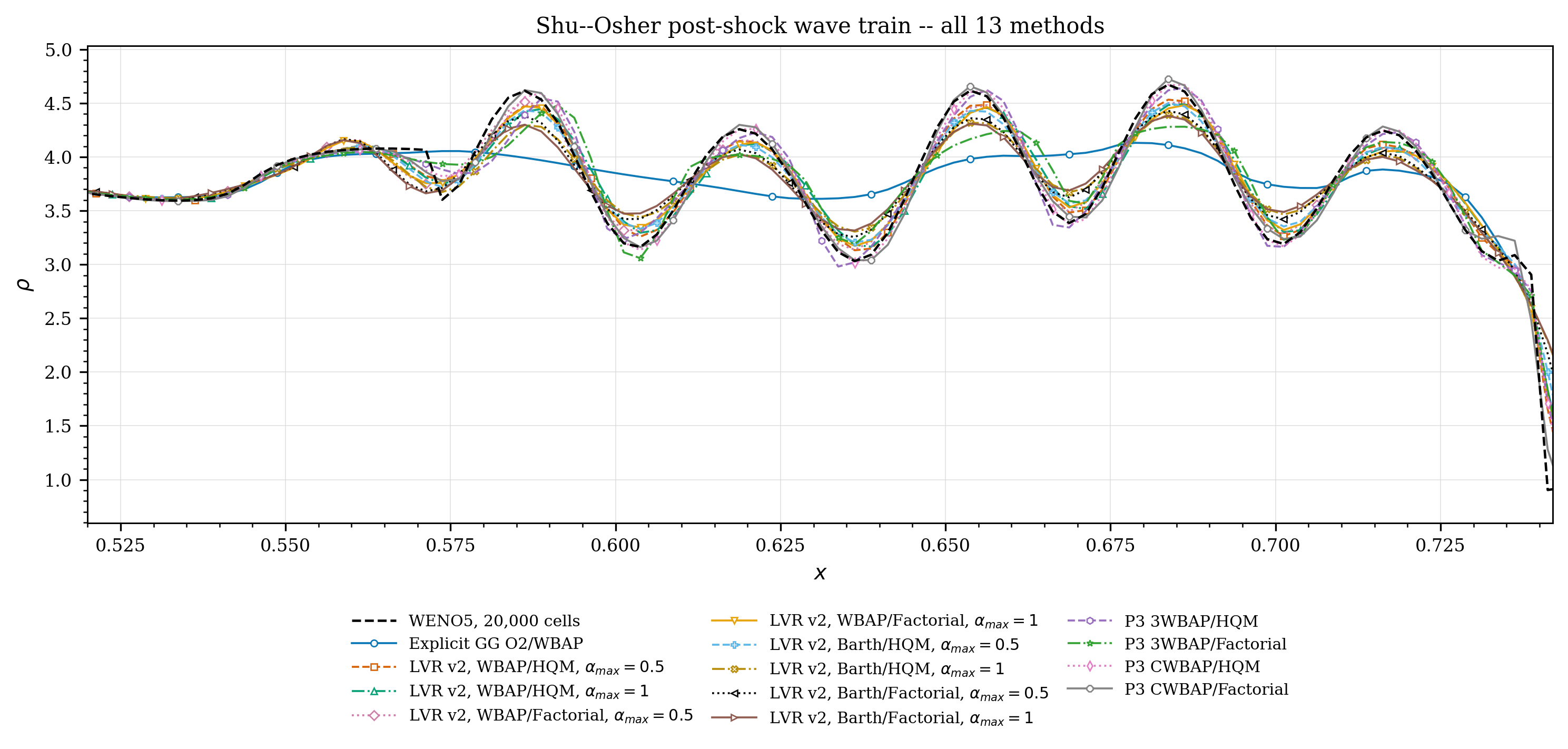 |
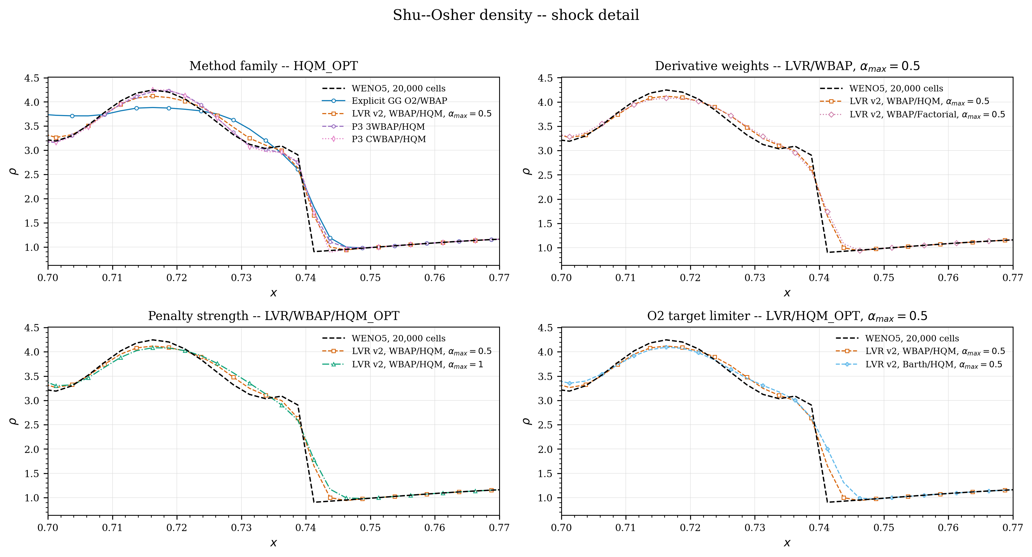
The separate all-method Shu–Osher shock-front detail is also retained:
Controlled $2\times2$ factor layouts
Each $2\times2$ figure uses the same four comparisons:
- Explicit O2, LVR v2, 3WBAP, and CWBAP with HQM_OPT weights;
- HQM_OPT versus Factorial derivative weights;
- LVR v2 with $\alpha_{max}=0.5$ versus $\alpha_{max}=1$;
- WBAP-based versus Barth-based LVR v2 O2 targets.
| Case | Full-view $2\times2$ layout | Detailed-view $2\times2$ layout |
|---|---|---|
| Mach-20 cylinder | 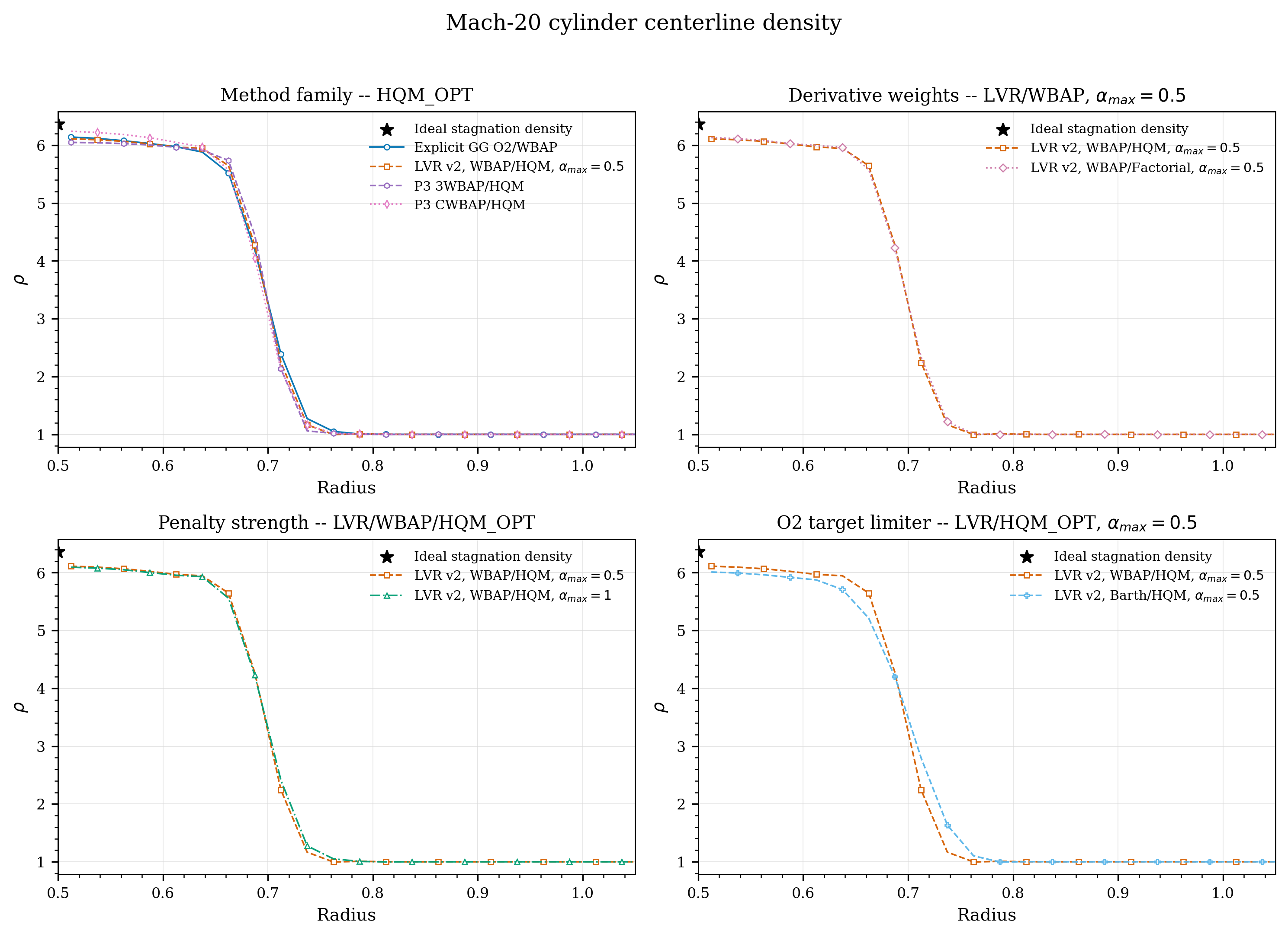 | 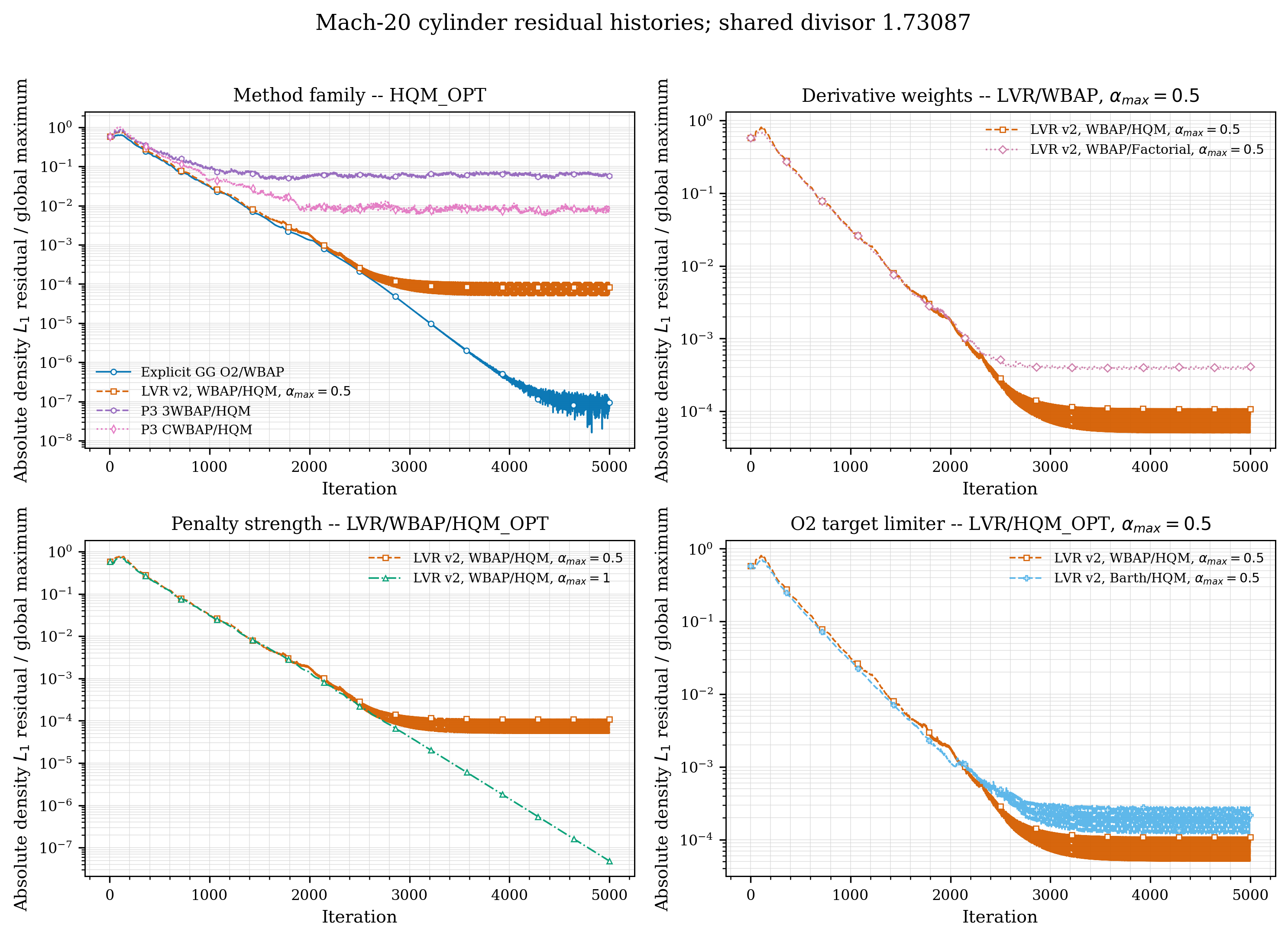 |
| Lax shock tube | 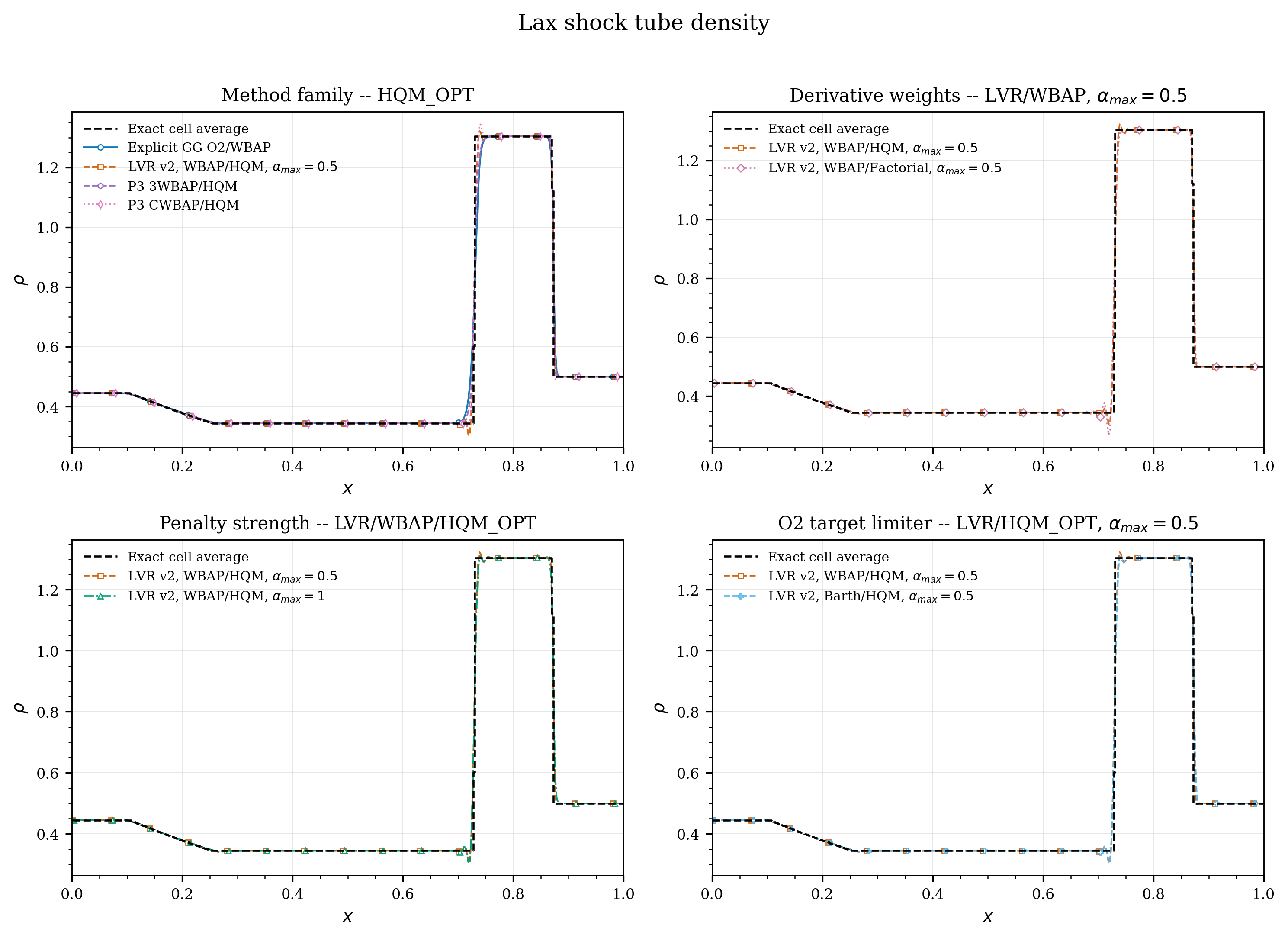 | 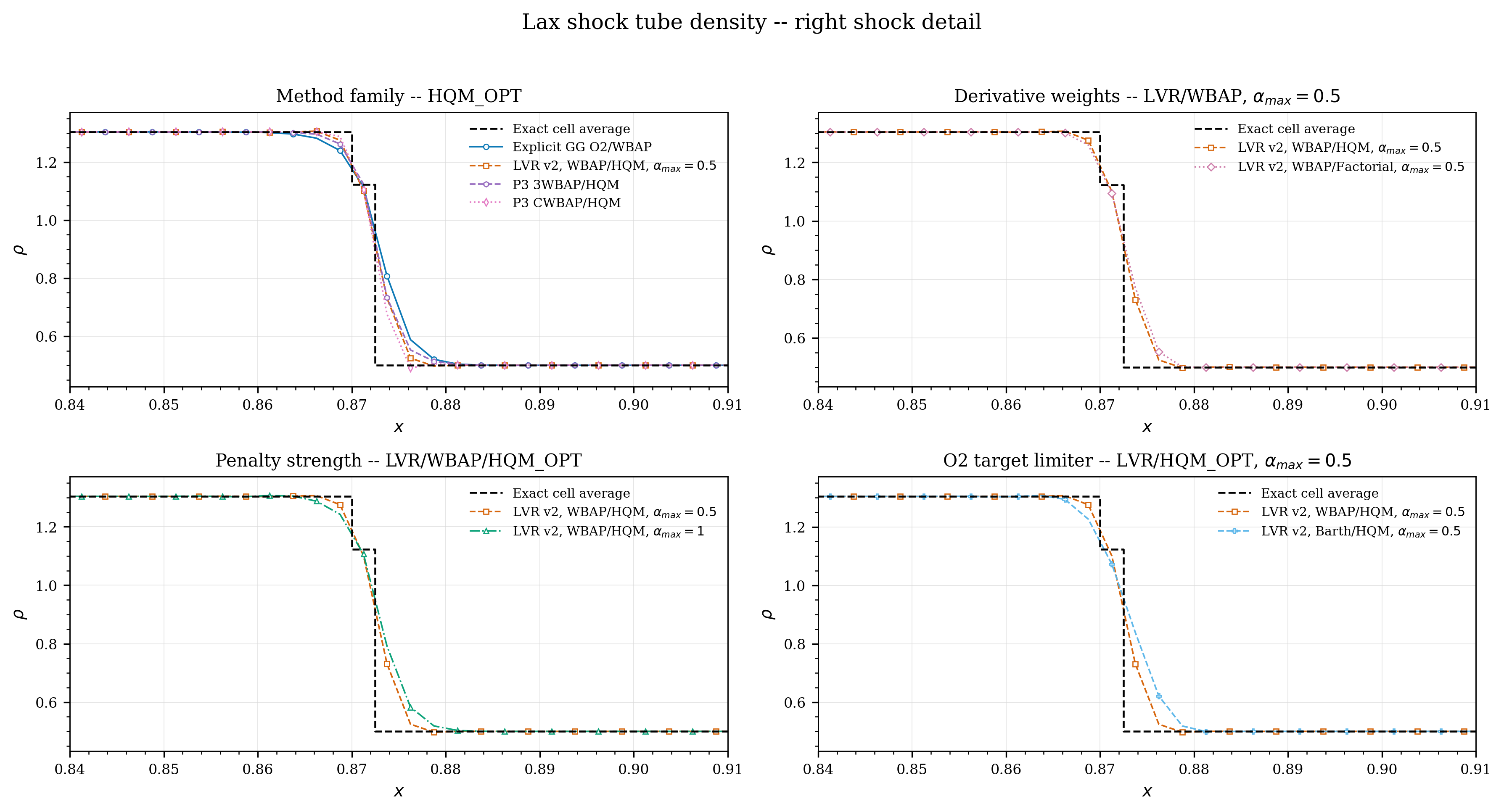 |
| Sod shock tube | 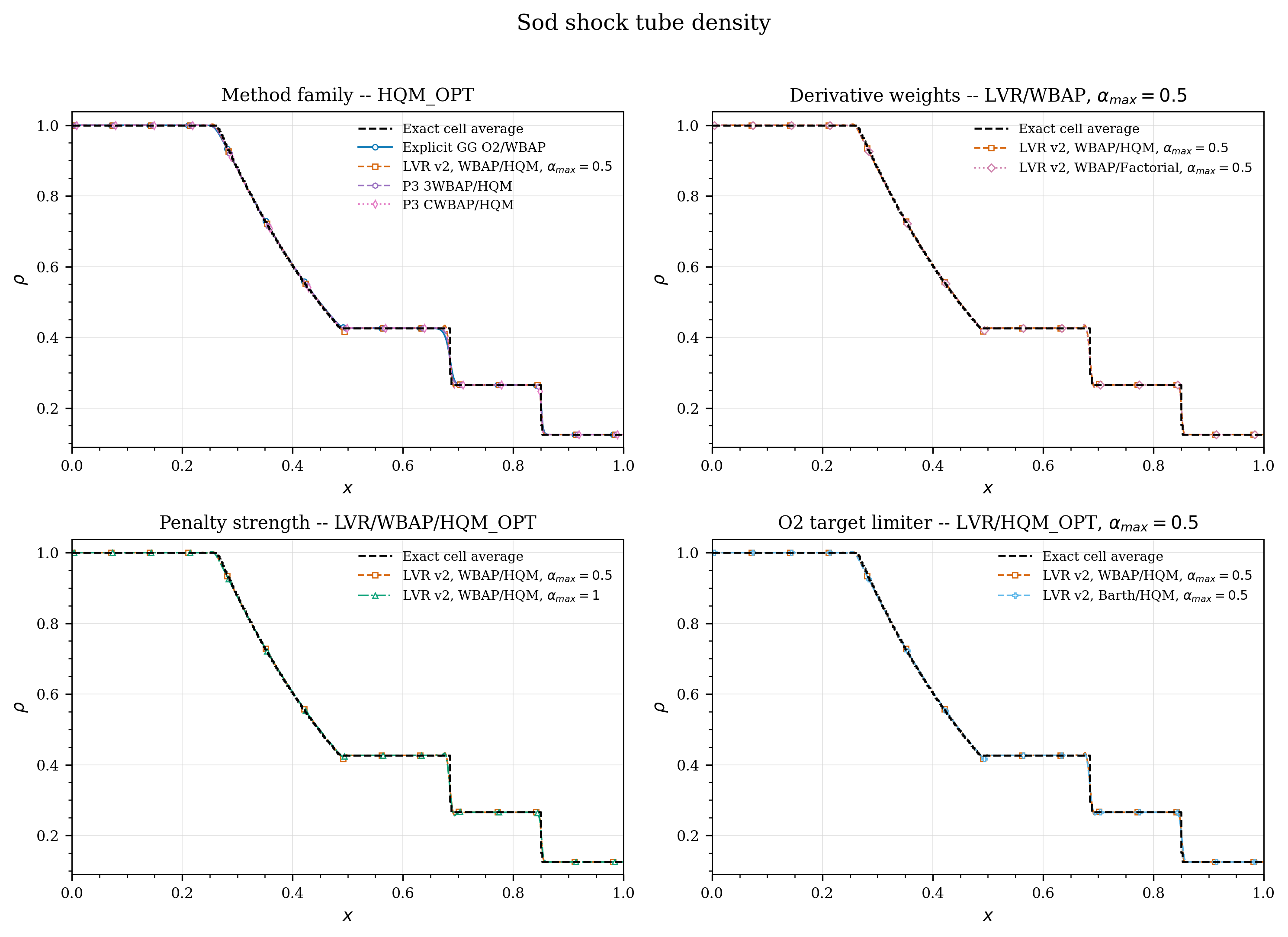 | 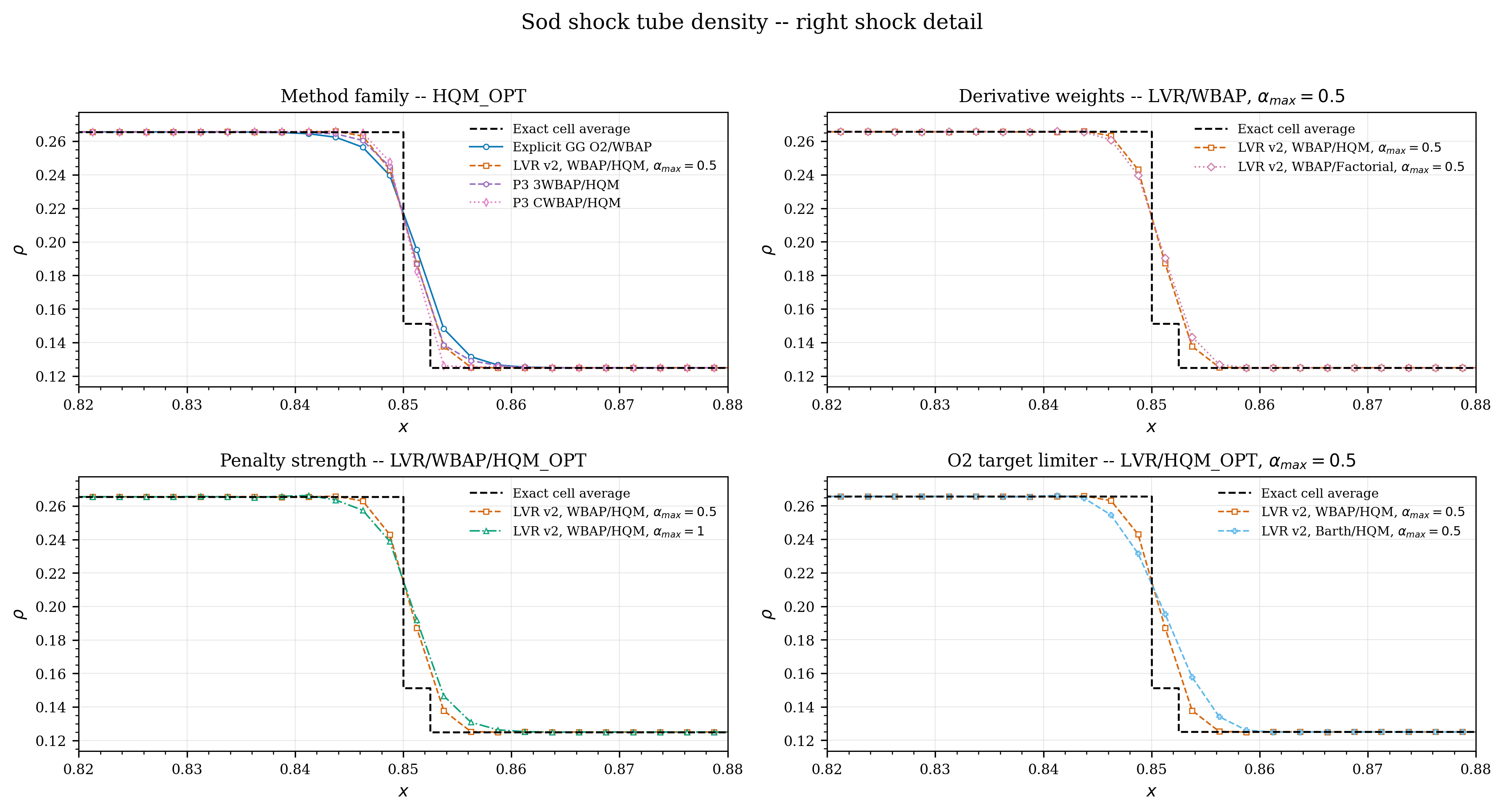 |
| Toro 123 double rarefaction | 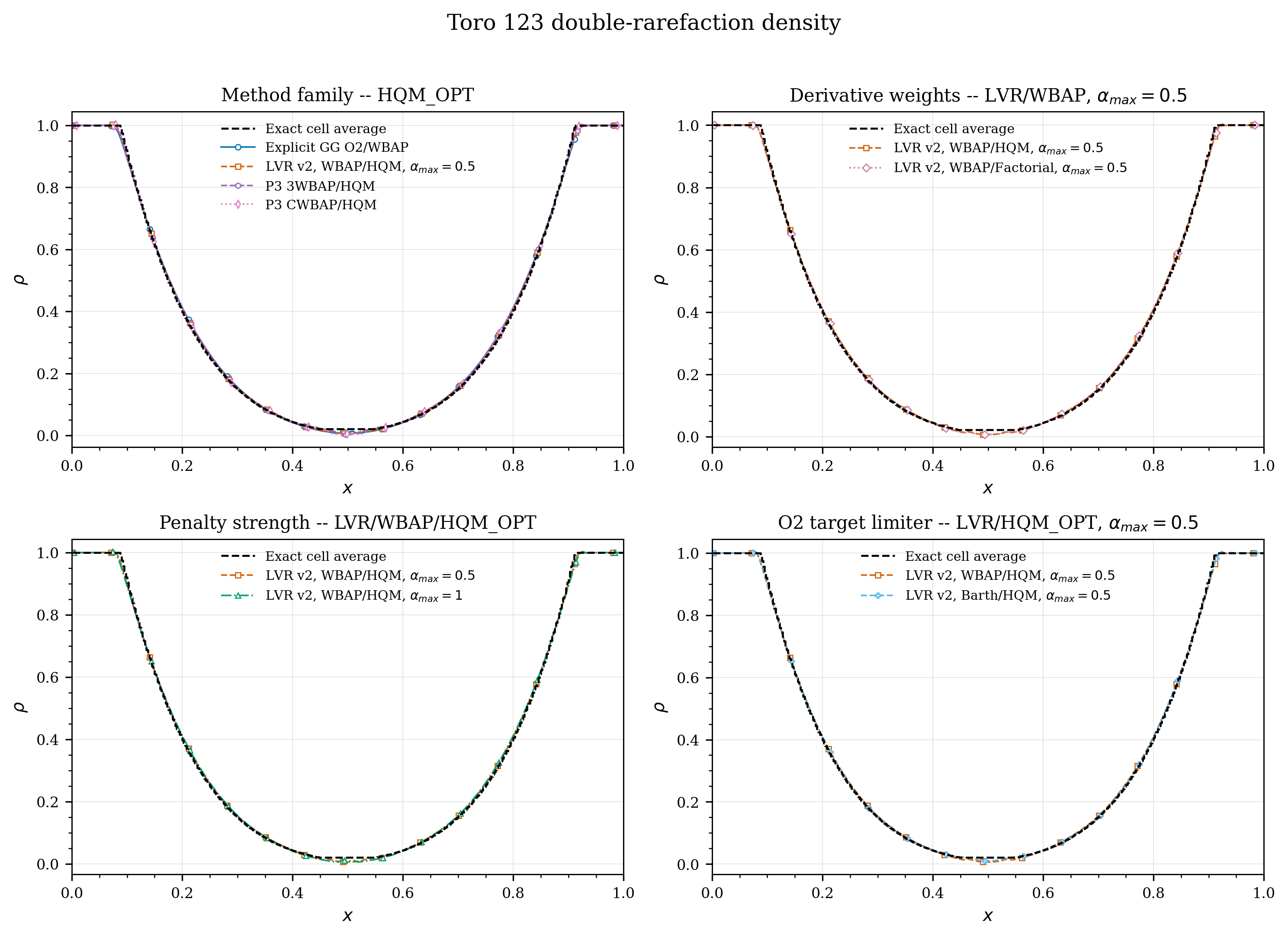 | 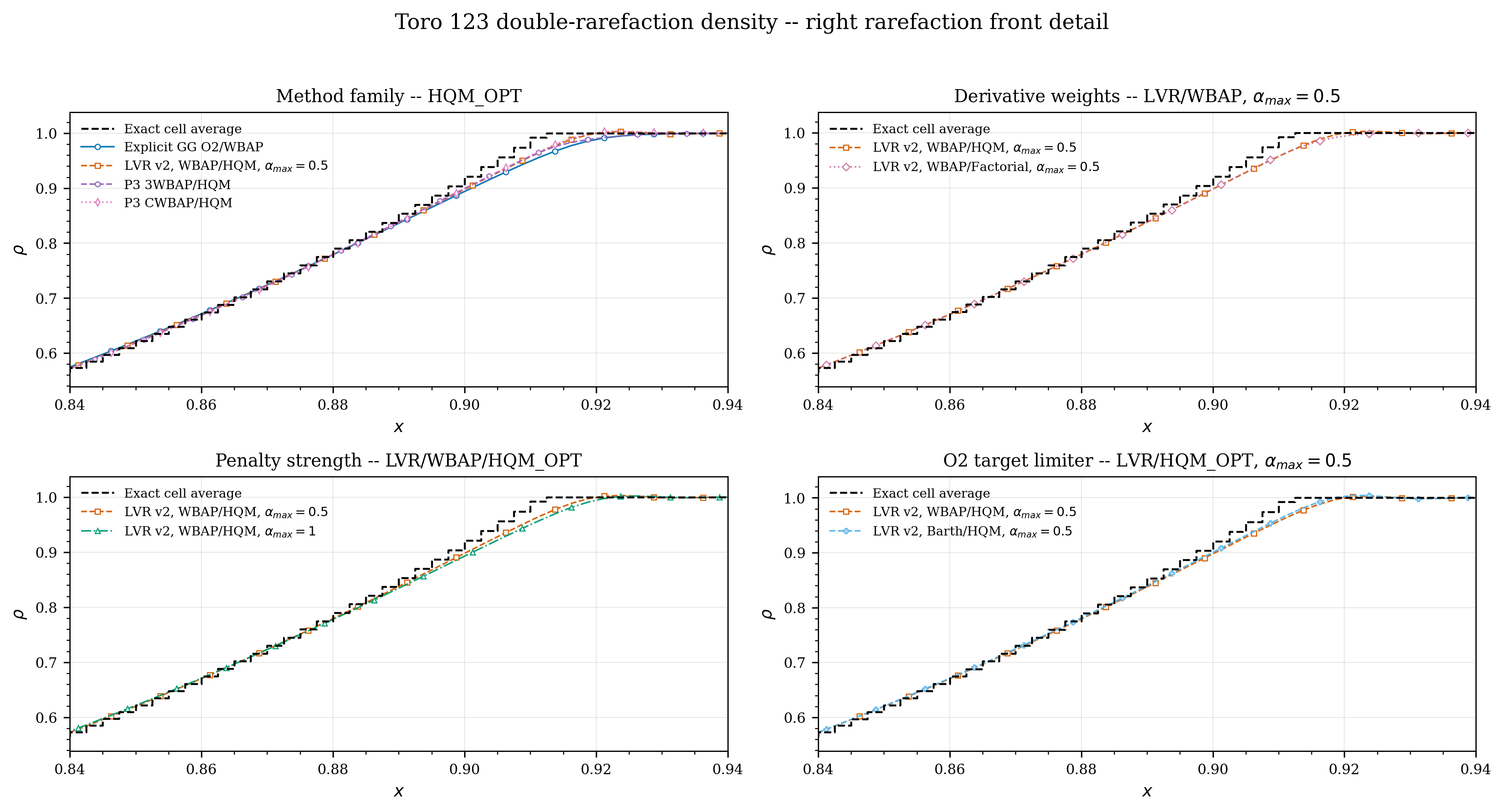 |
| Two-shock problem | 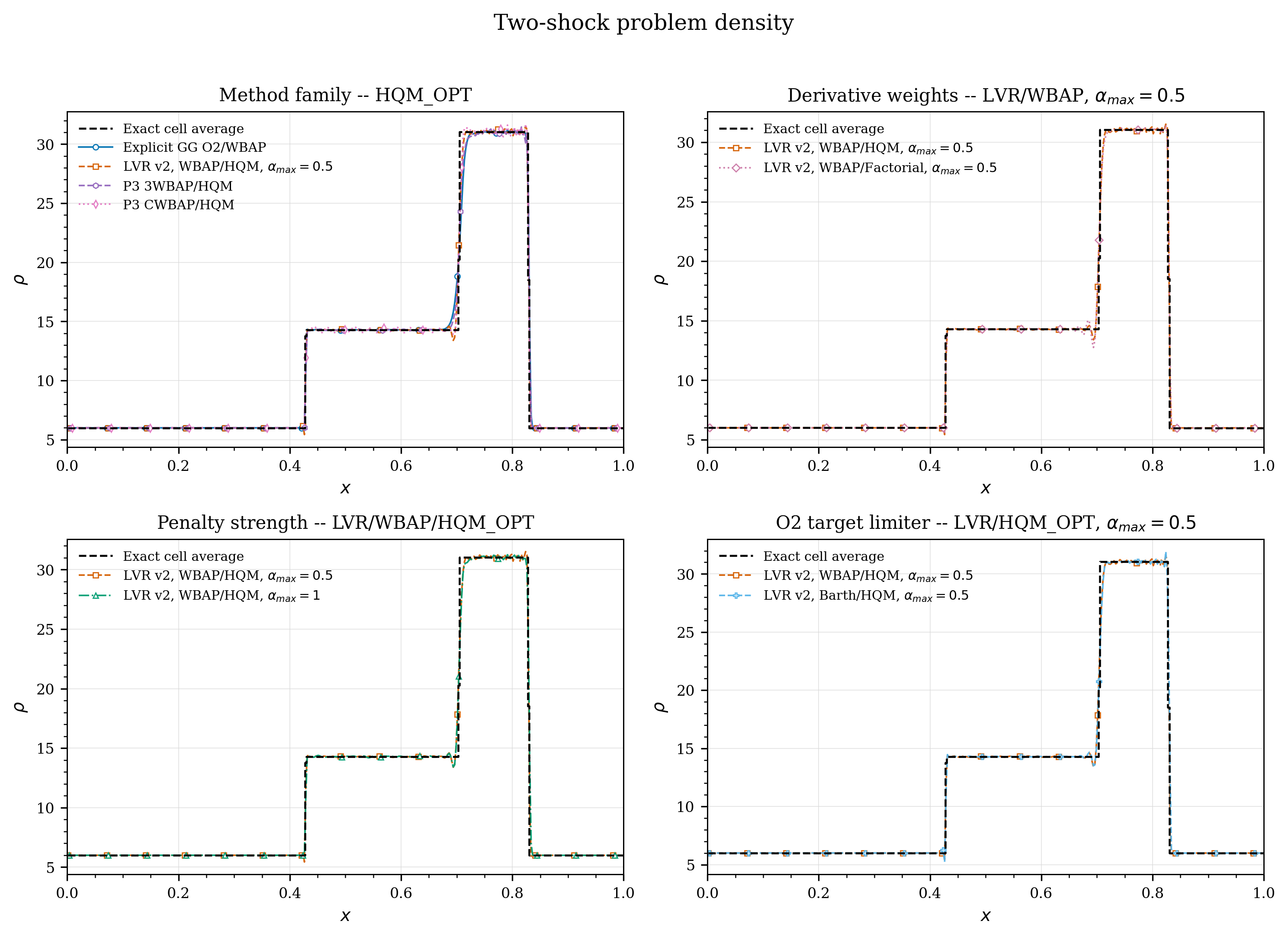 | 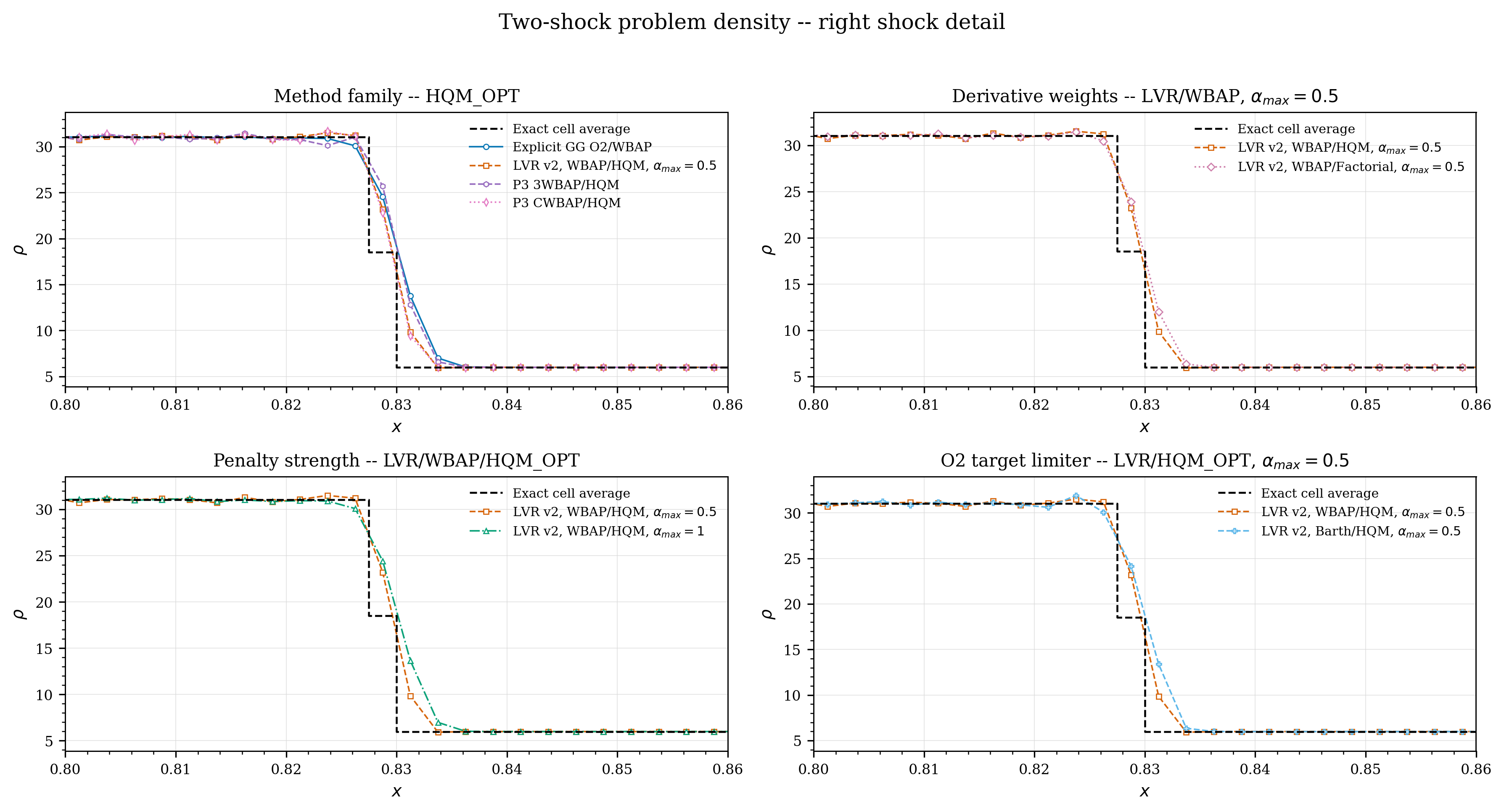 |
| Shu–Osher | 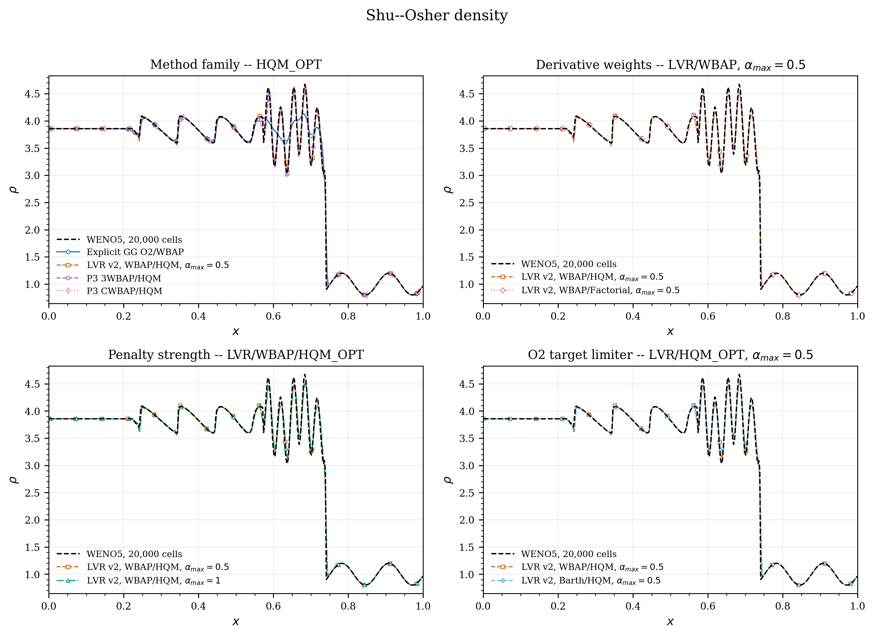 | 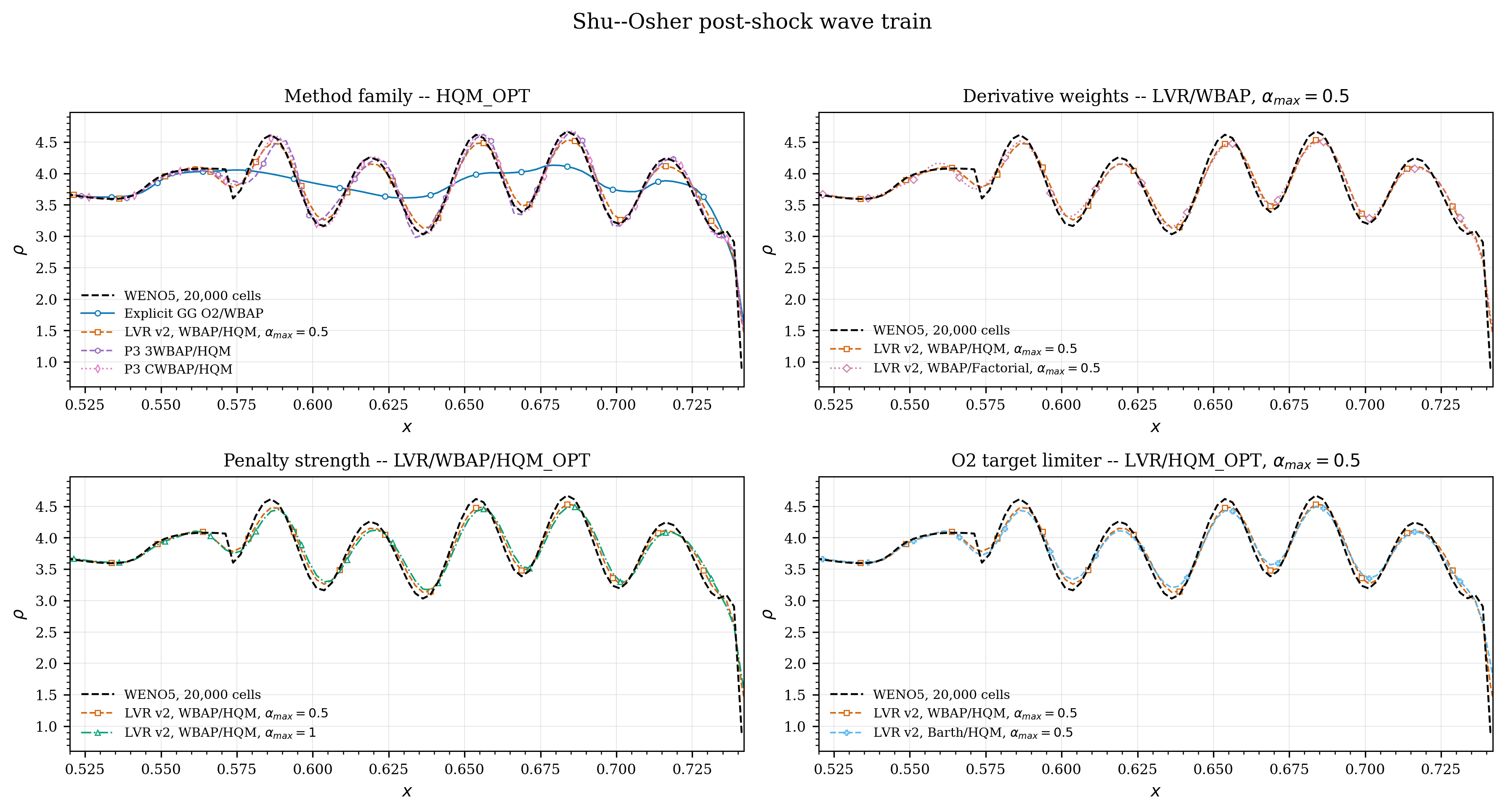 |
The separate $2\times2$ Shu–Osher shock-front detail is:
Reading the matrix
The principal observations are:
- Explicit O2 is robust but visibly diffusive.
- WBAP/HQM_OPT LVR v2 with $\alpha_{max}=0.5$ gives the flattest selected Lax downstream state while remaining sharper than Explicit O2.
- Barth-based targets broaden strong shocks more visibly.
- High-order LVR and conventional P3 limiters preserve substantially more Shu–Osher wave amplitude than Explicit O2.
- The cylinder residual histories separate methods whose final centerline profiles look similar but whose convergence floors differ substantially.
Double Mach reflection
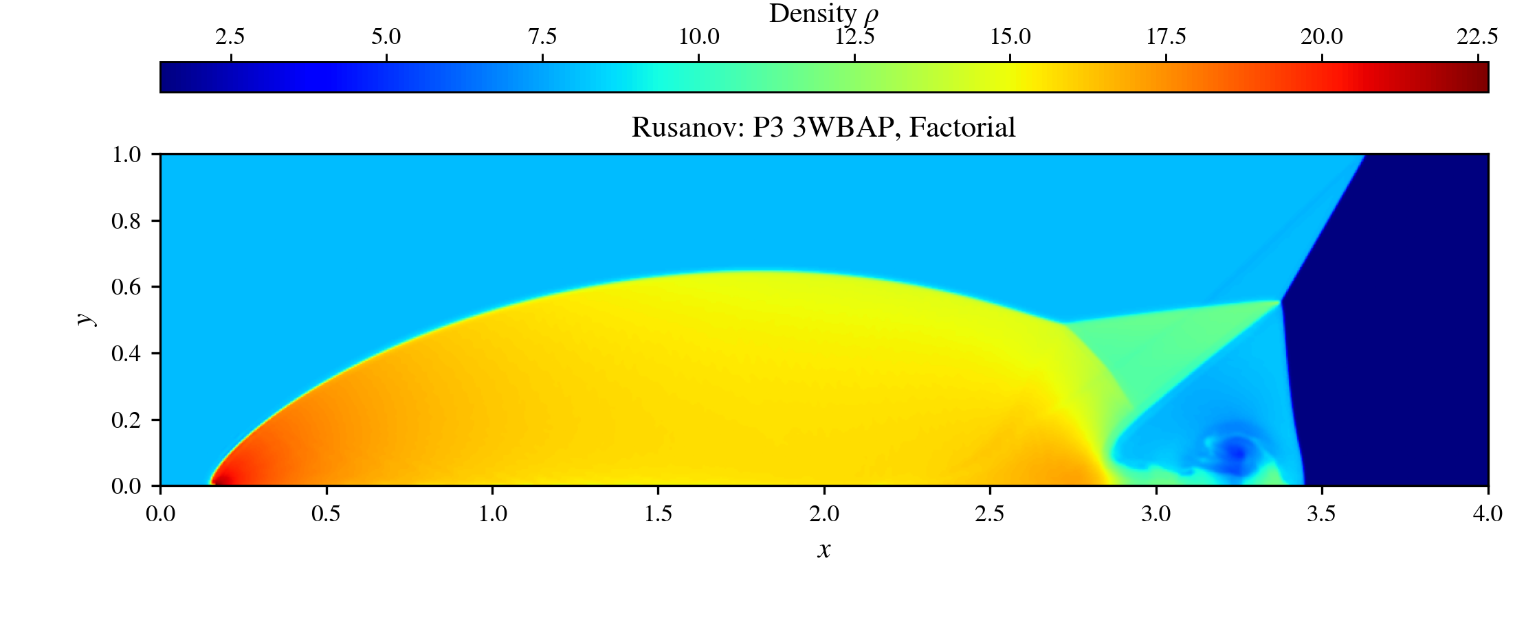
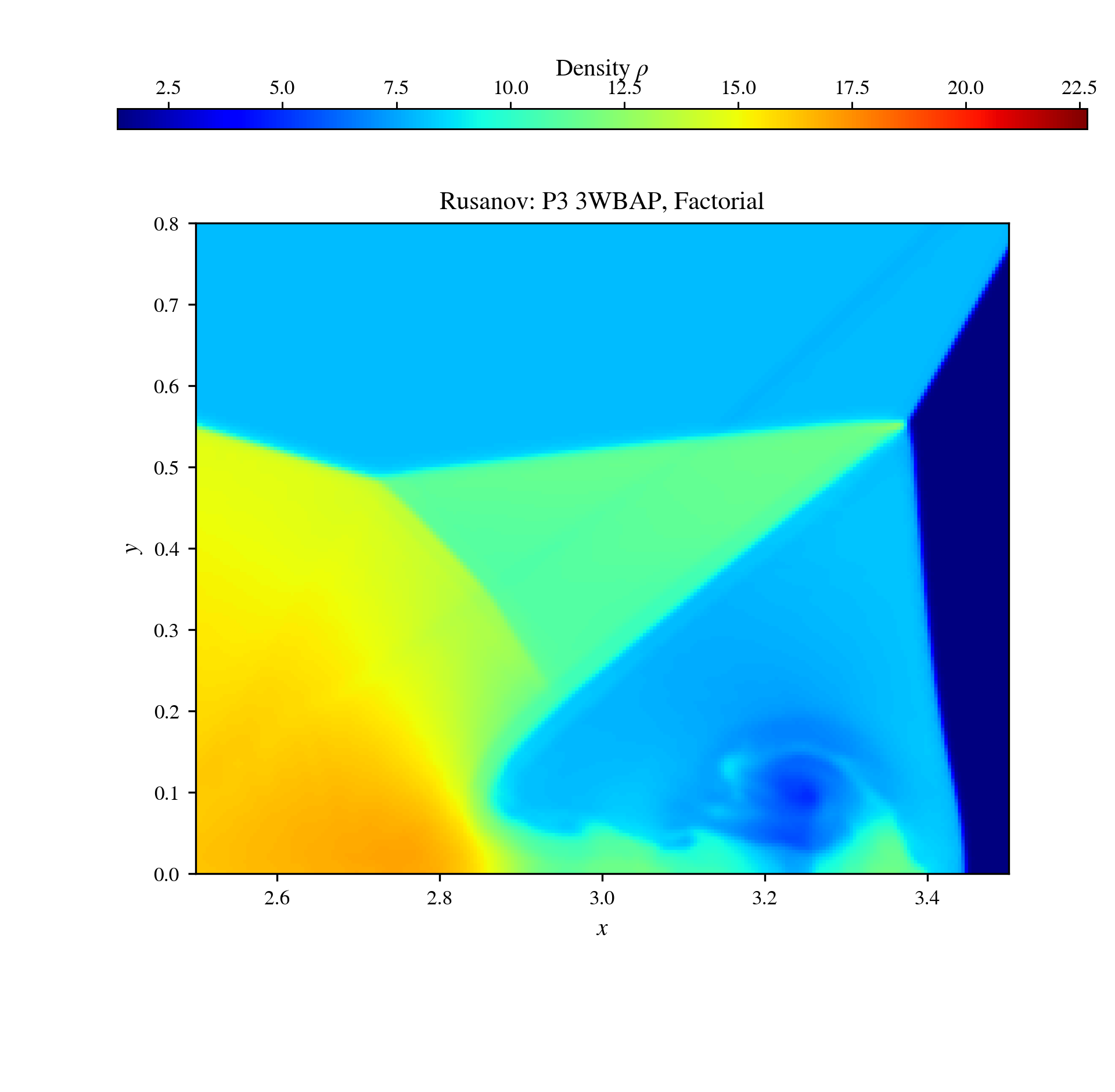
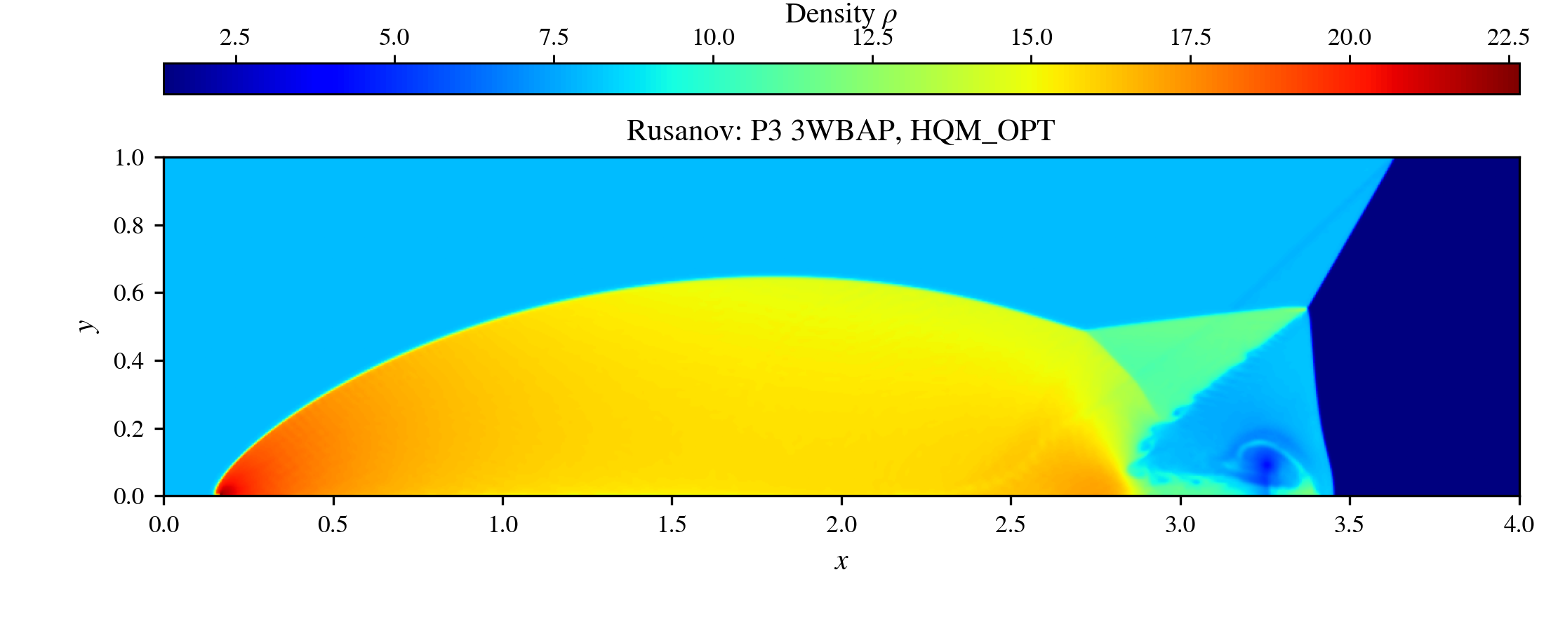
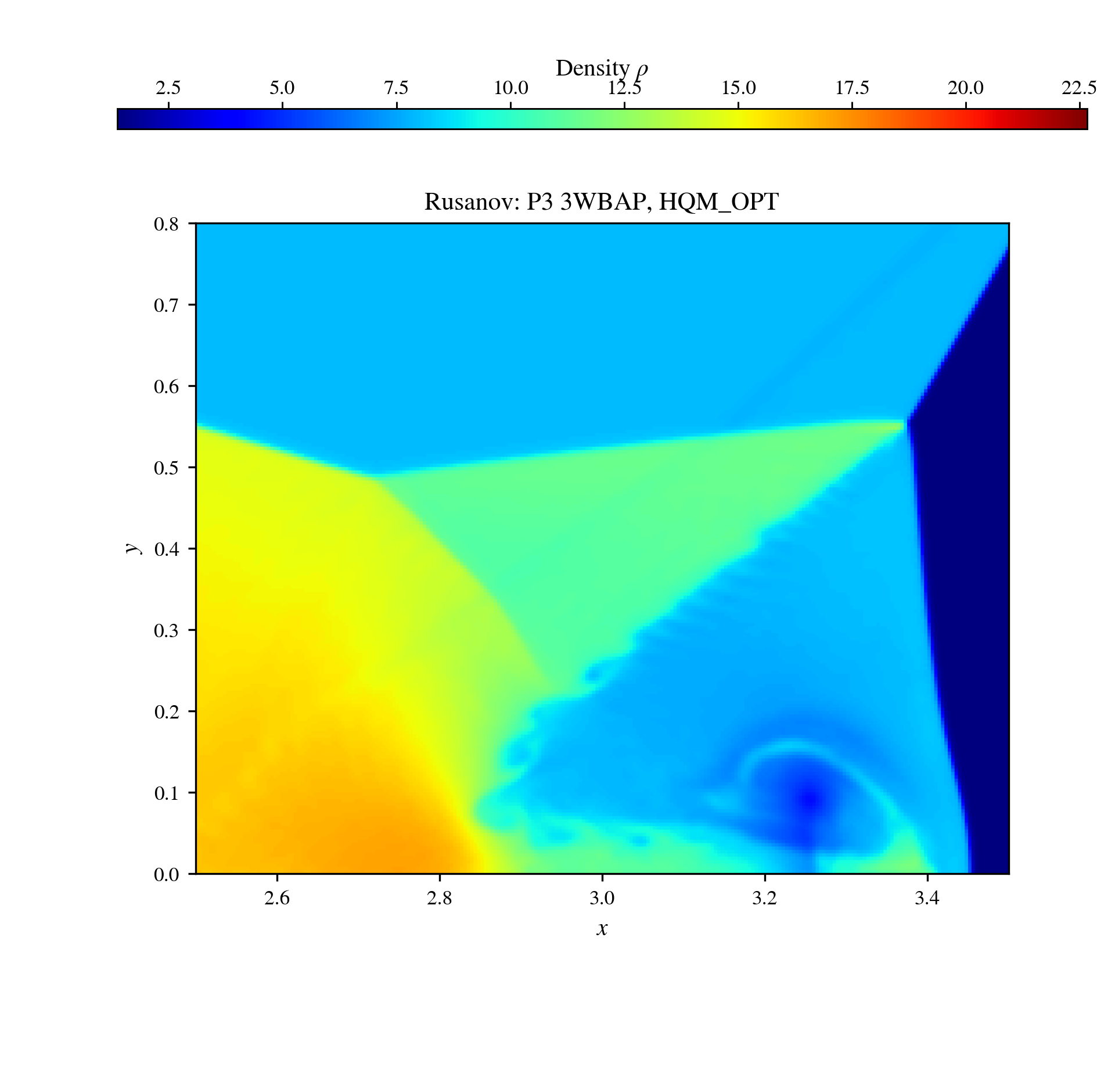
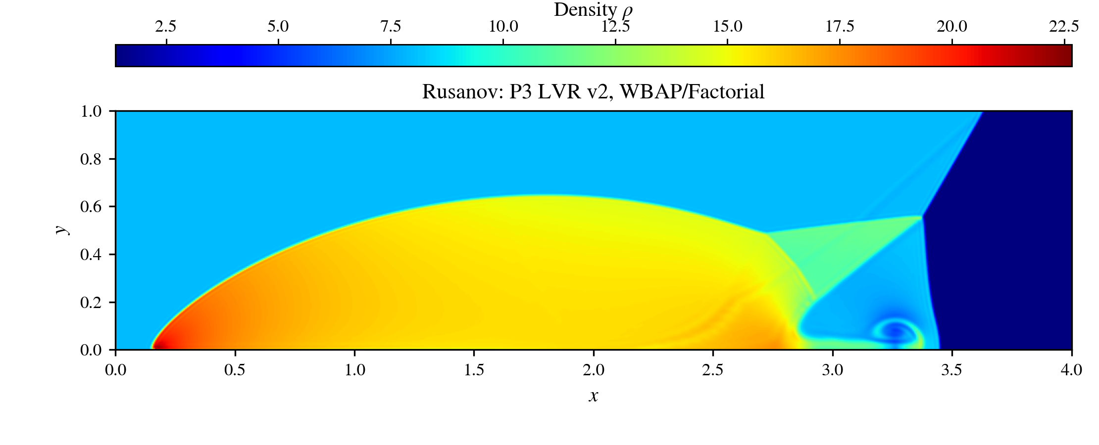
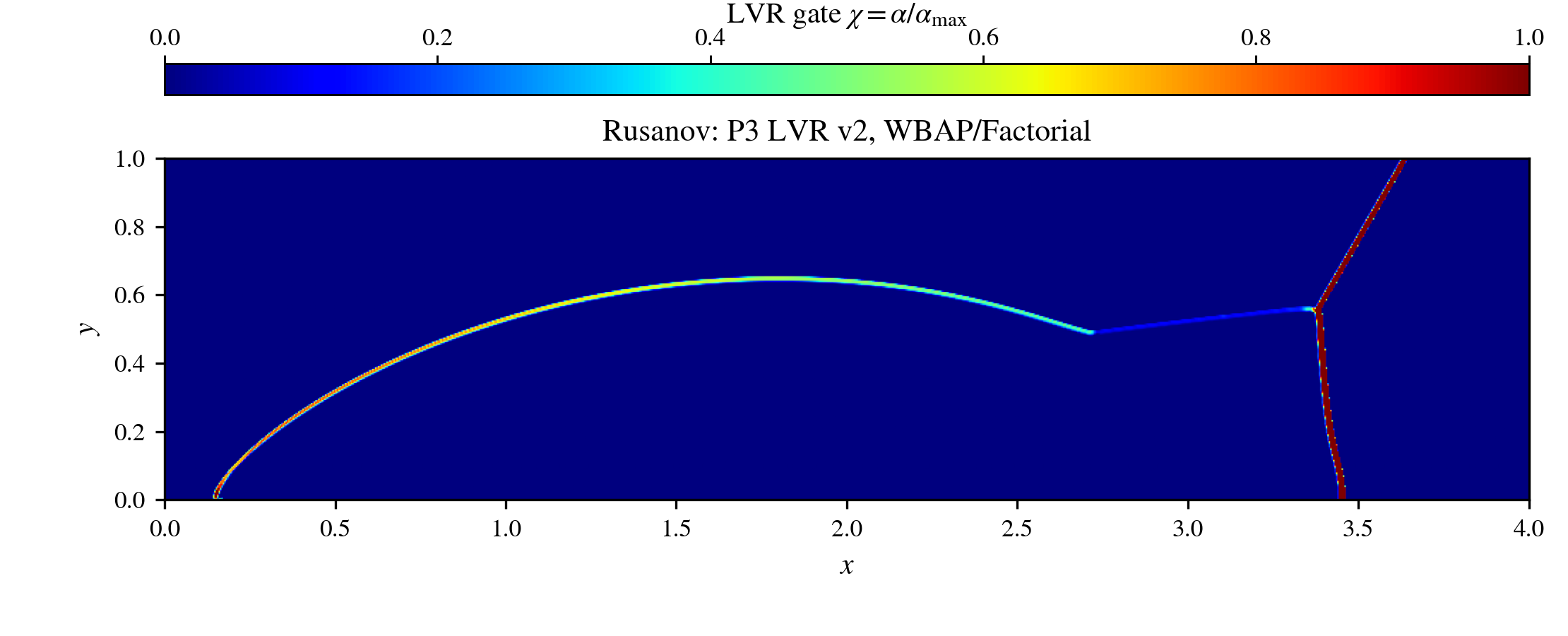
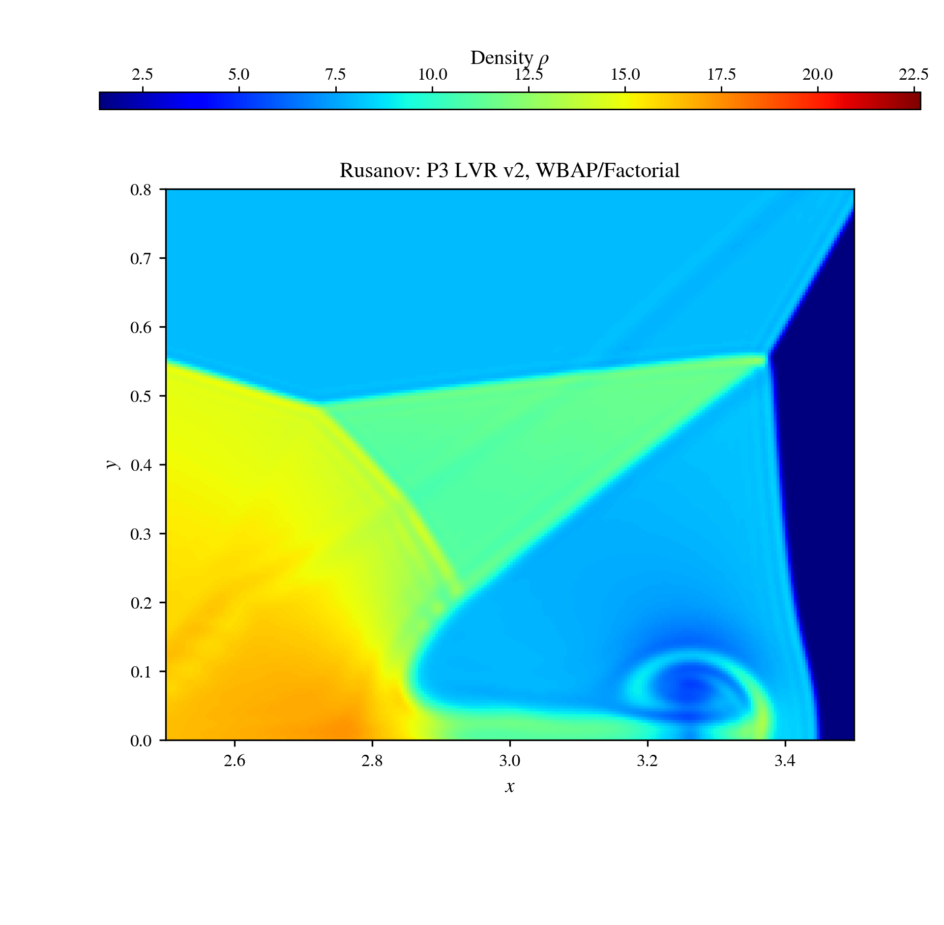
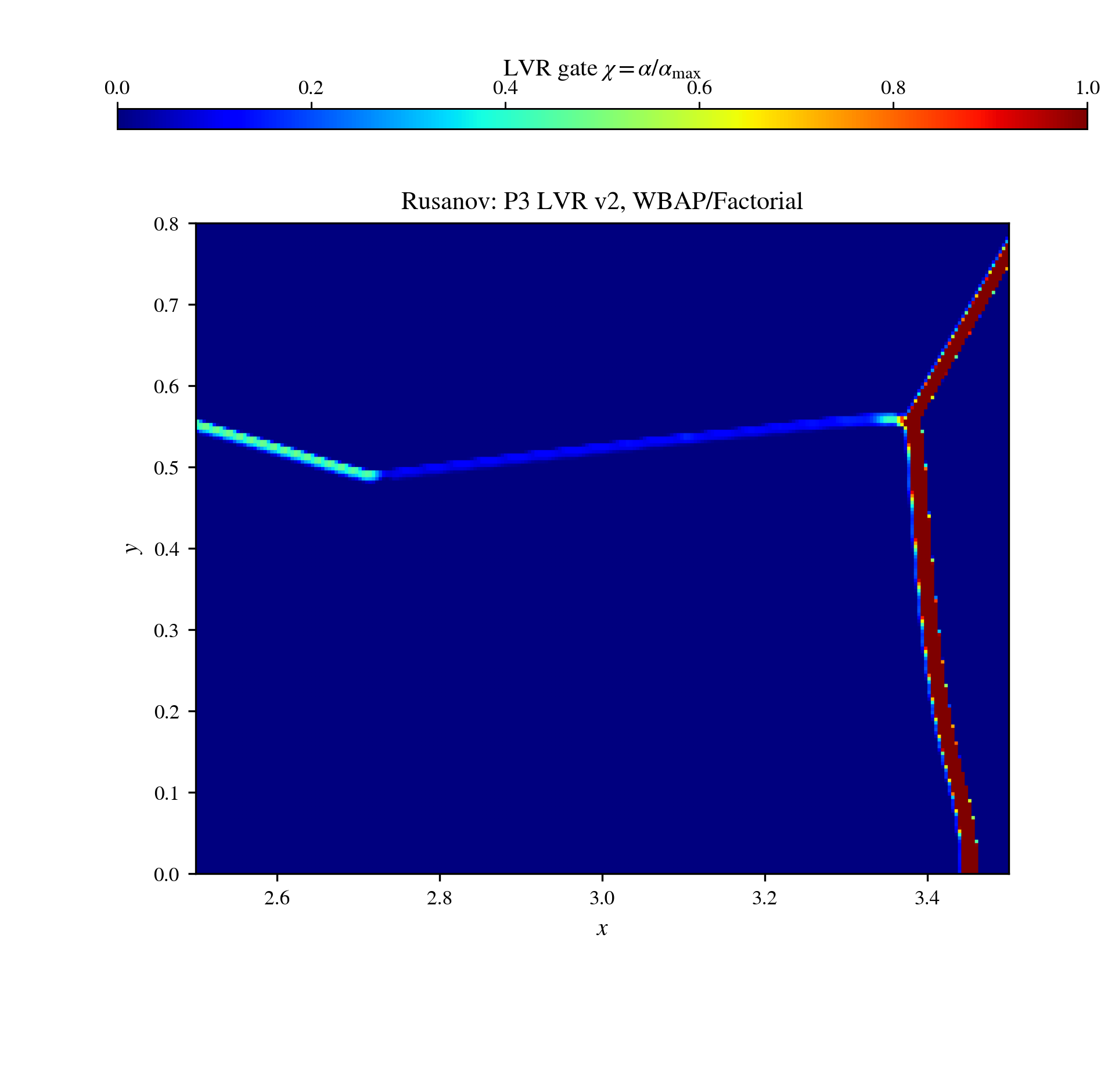
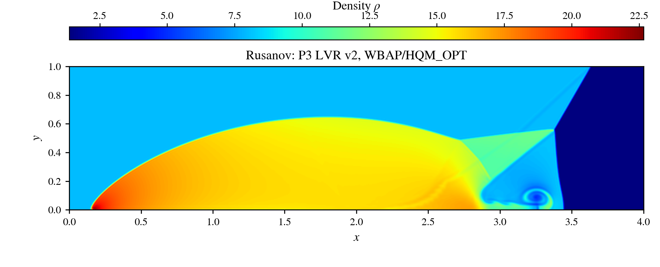
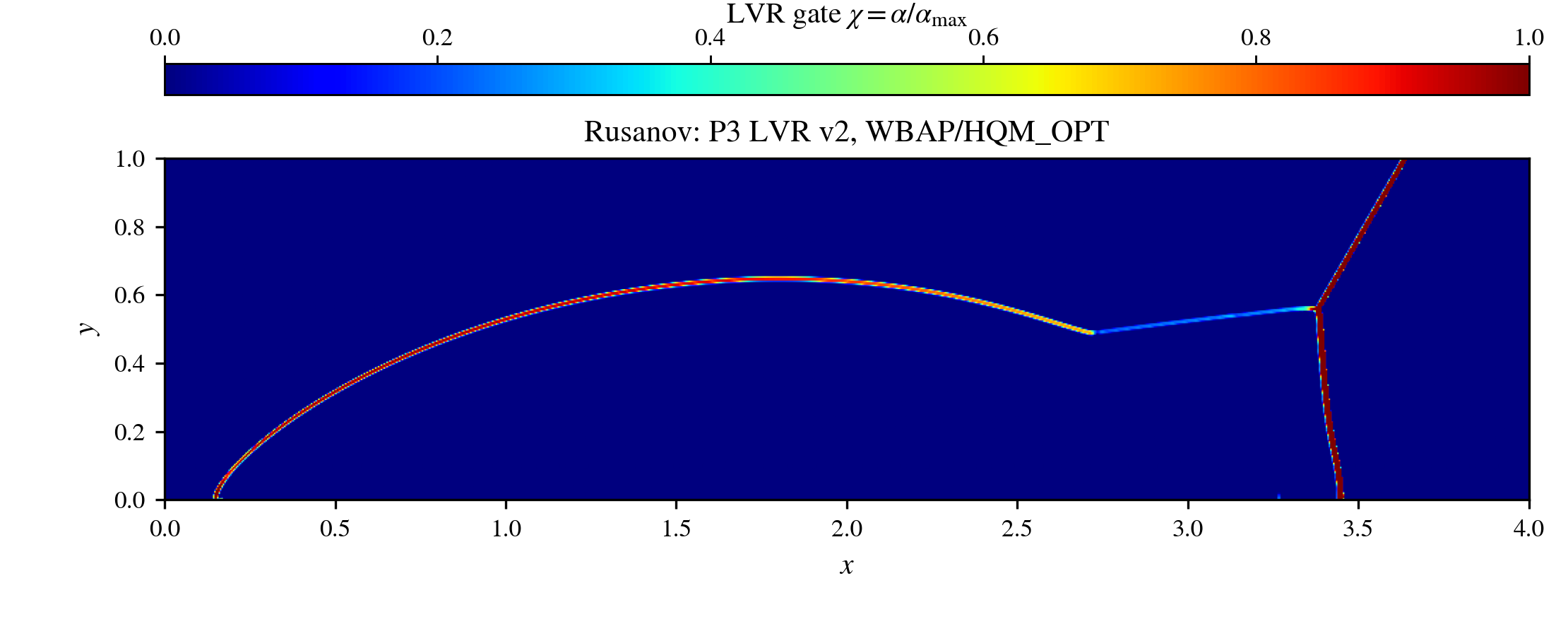
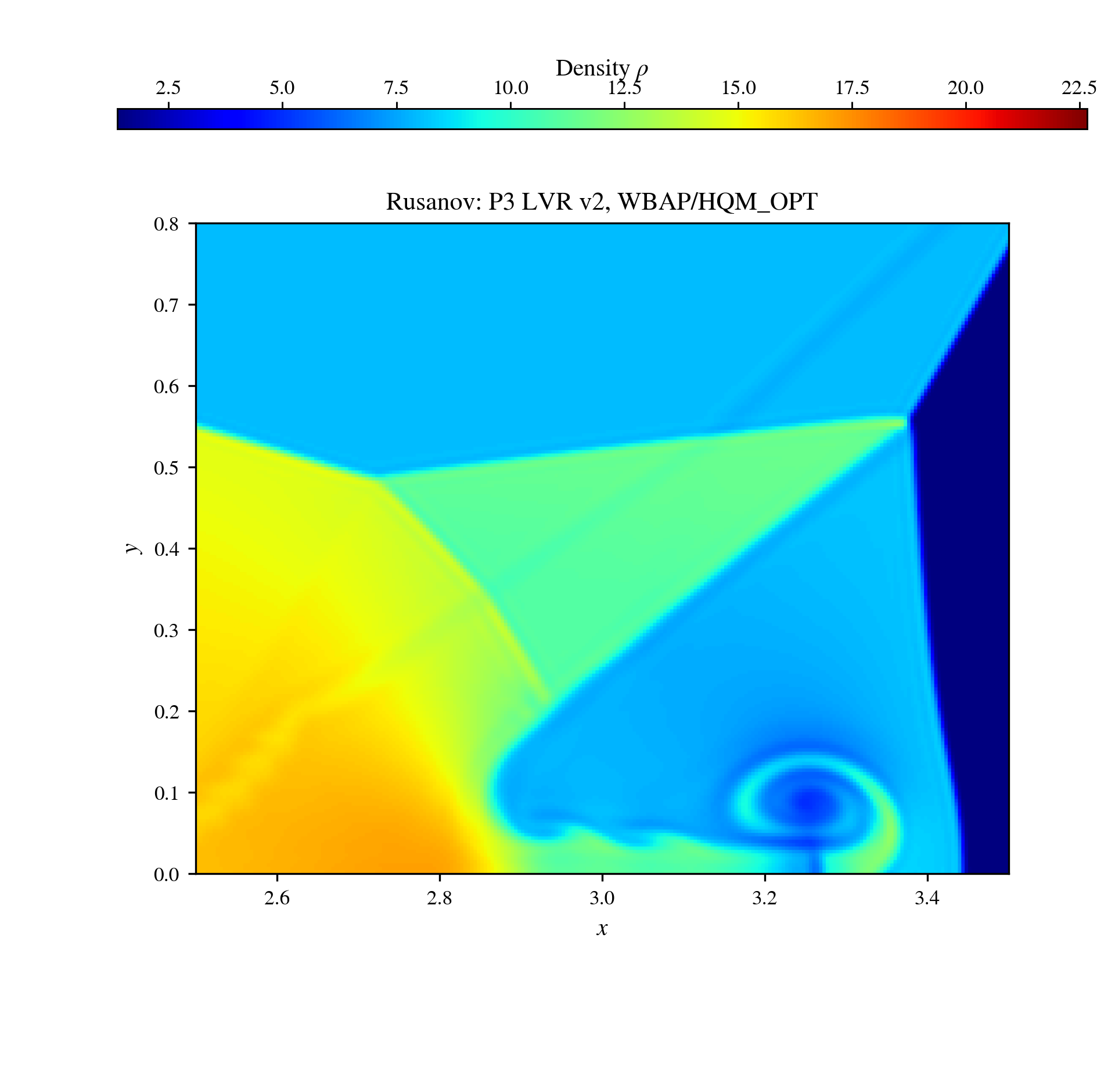
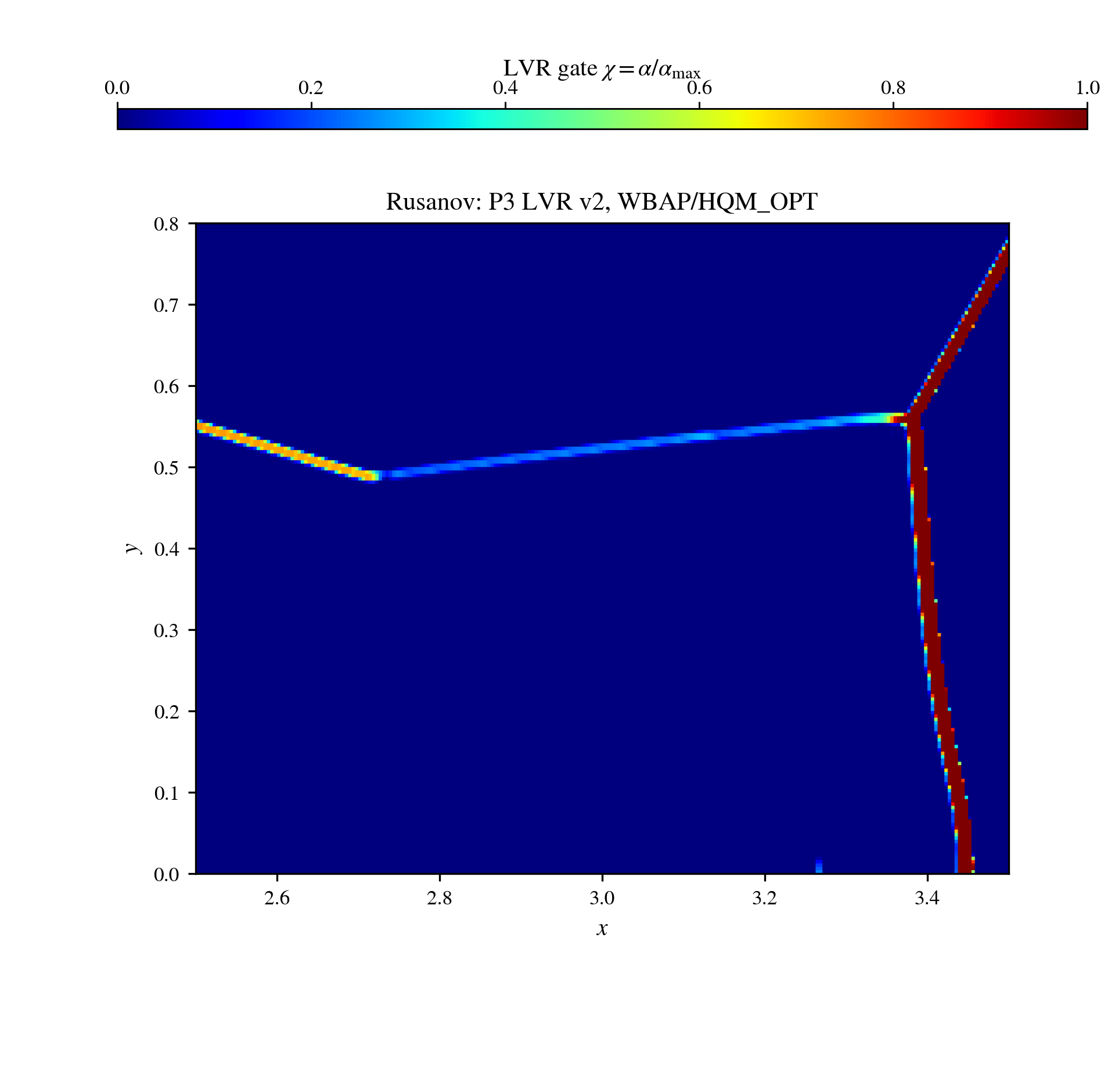
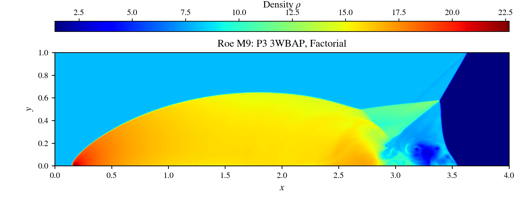
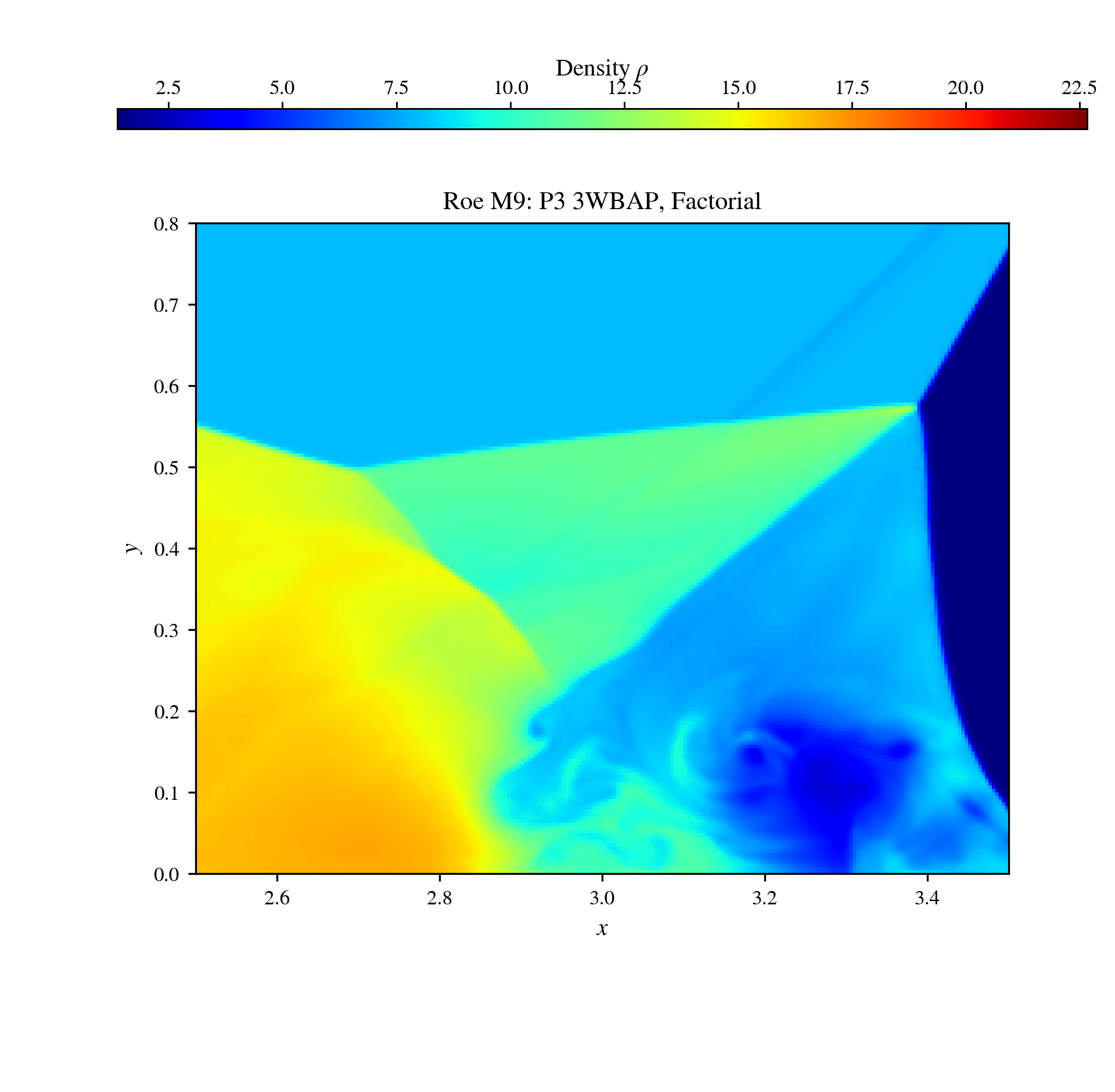
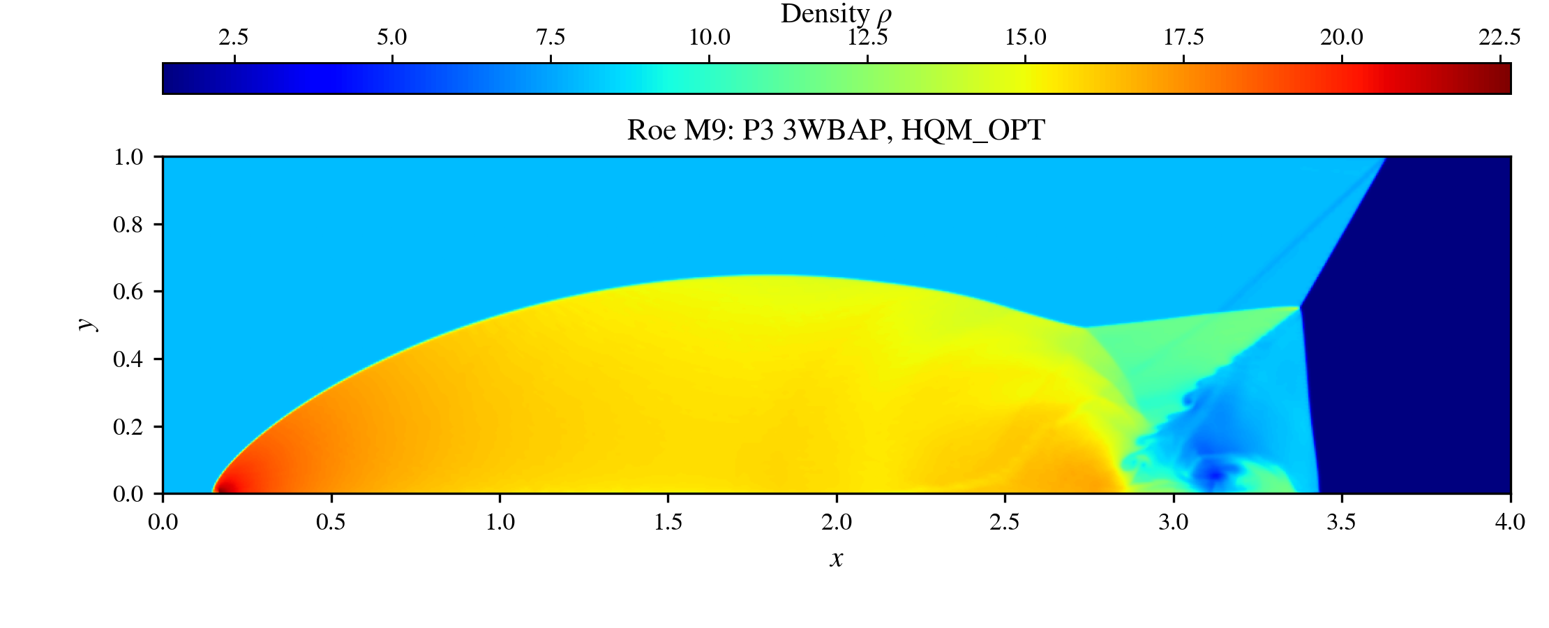
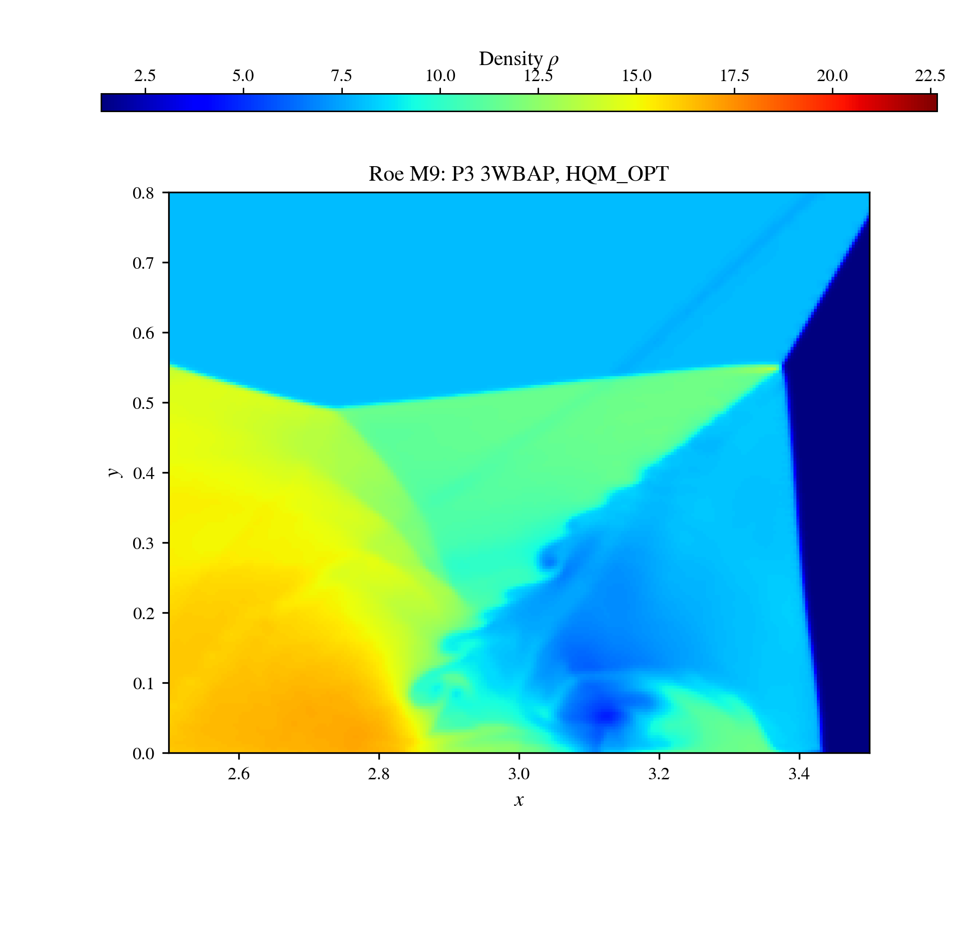
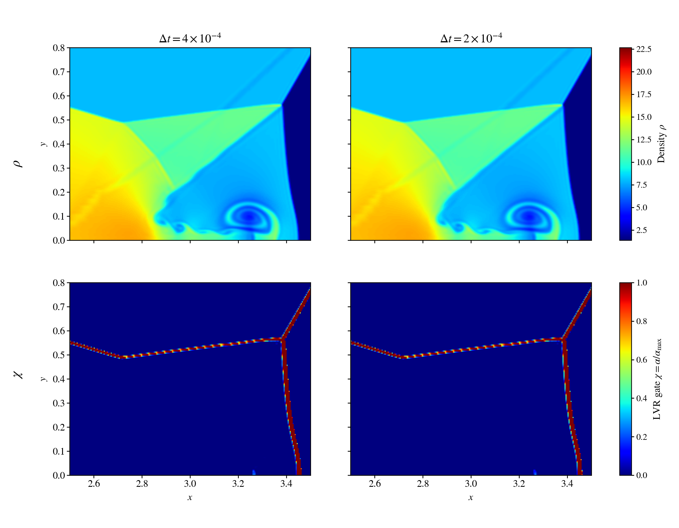
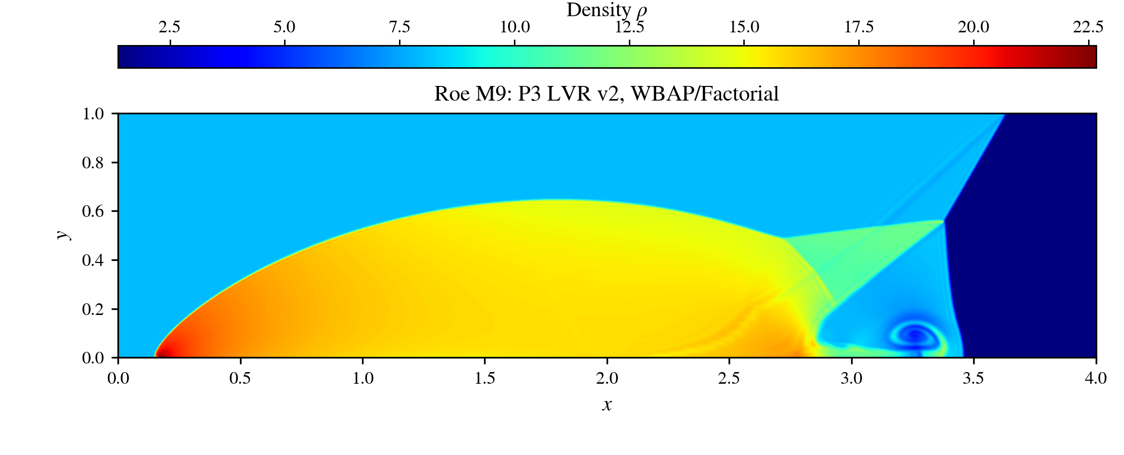
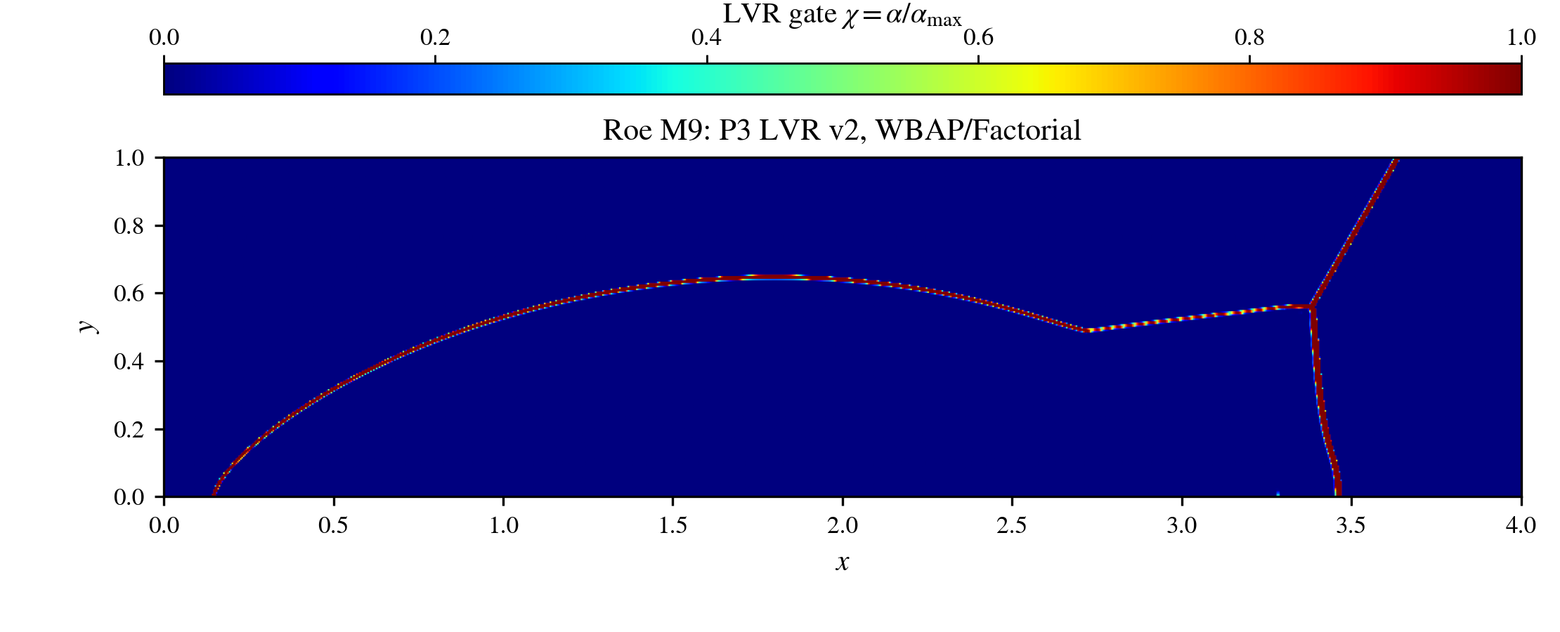
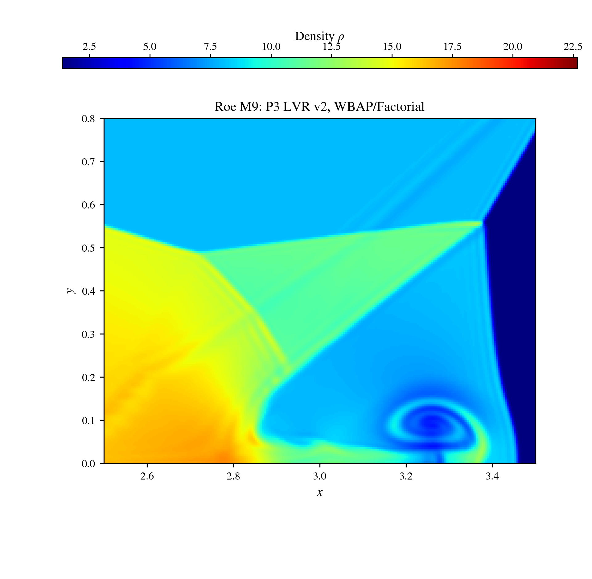
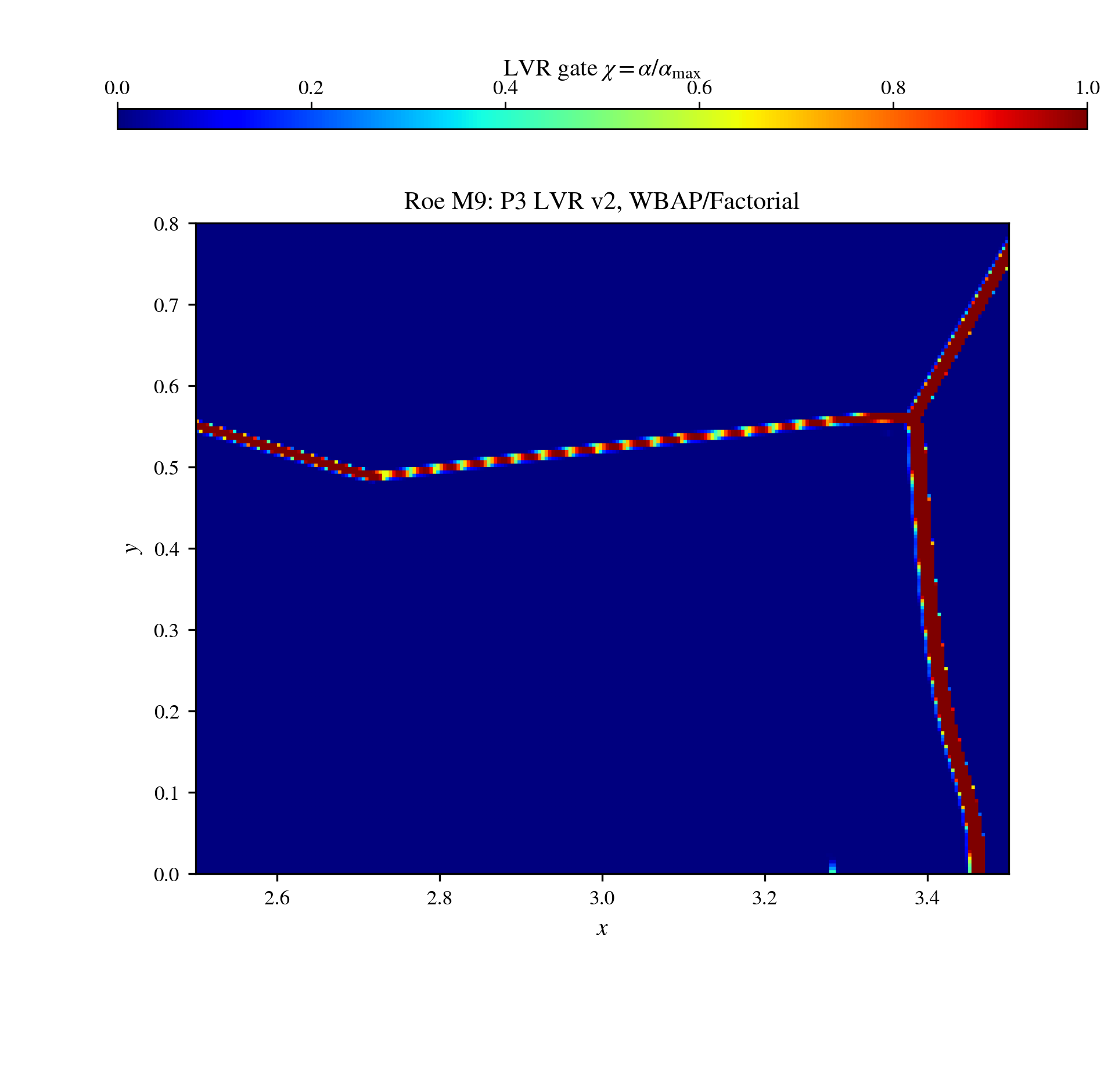
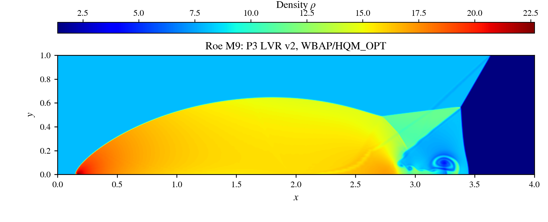
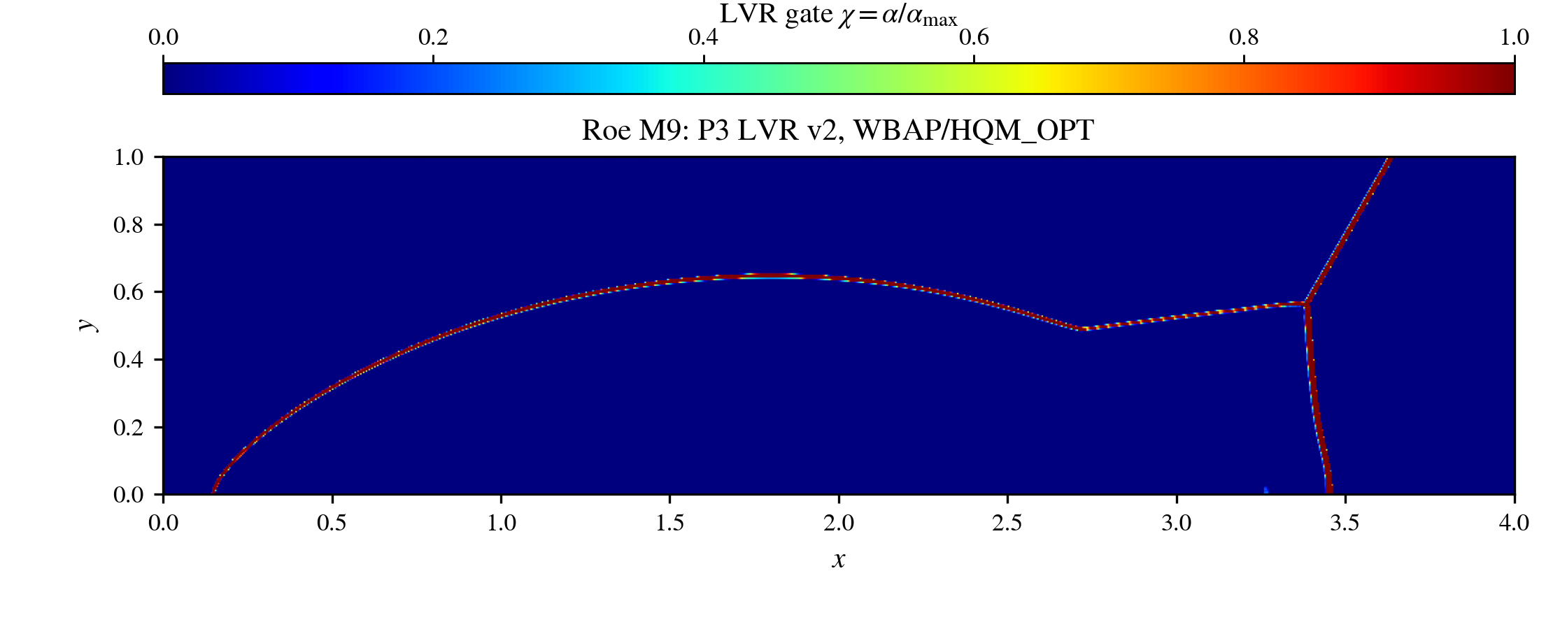
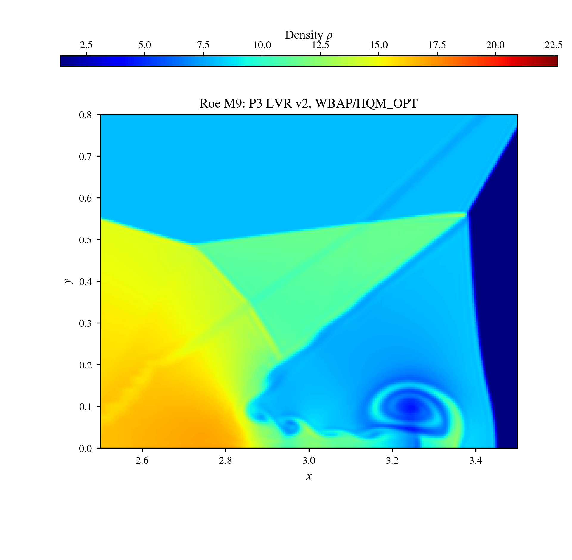
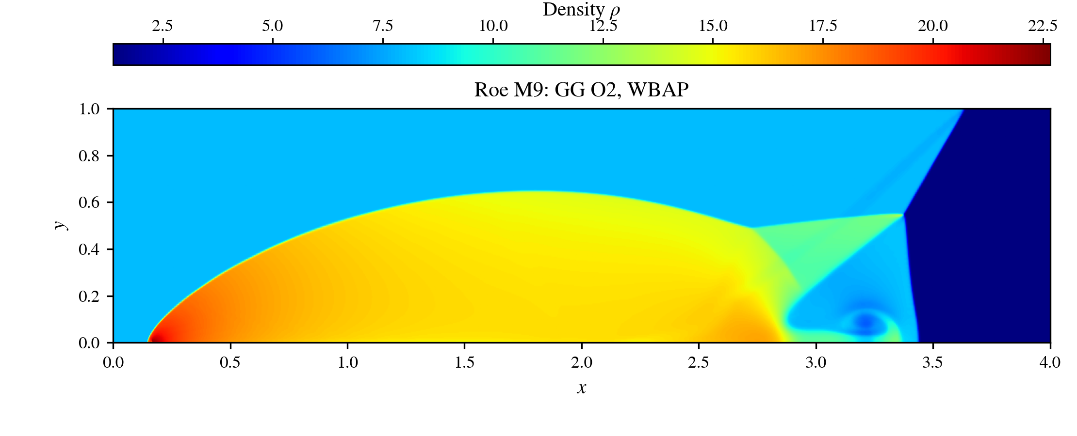
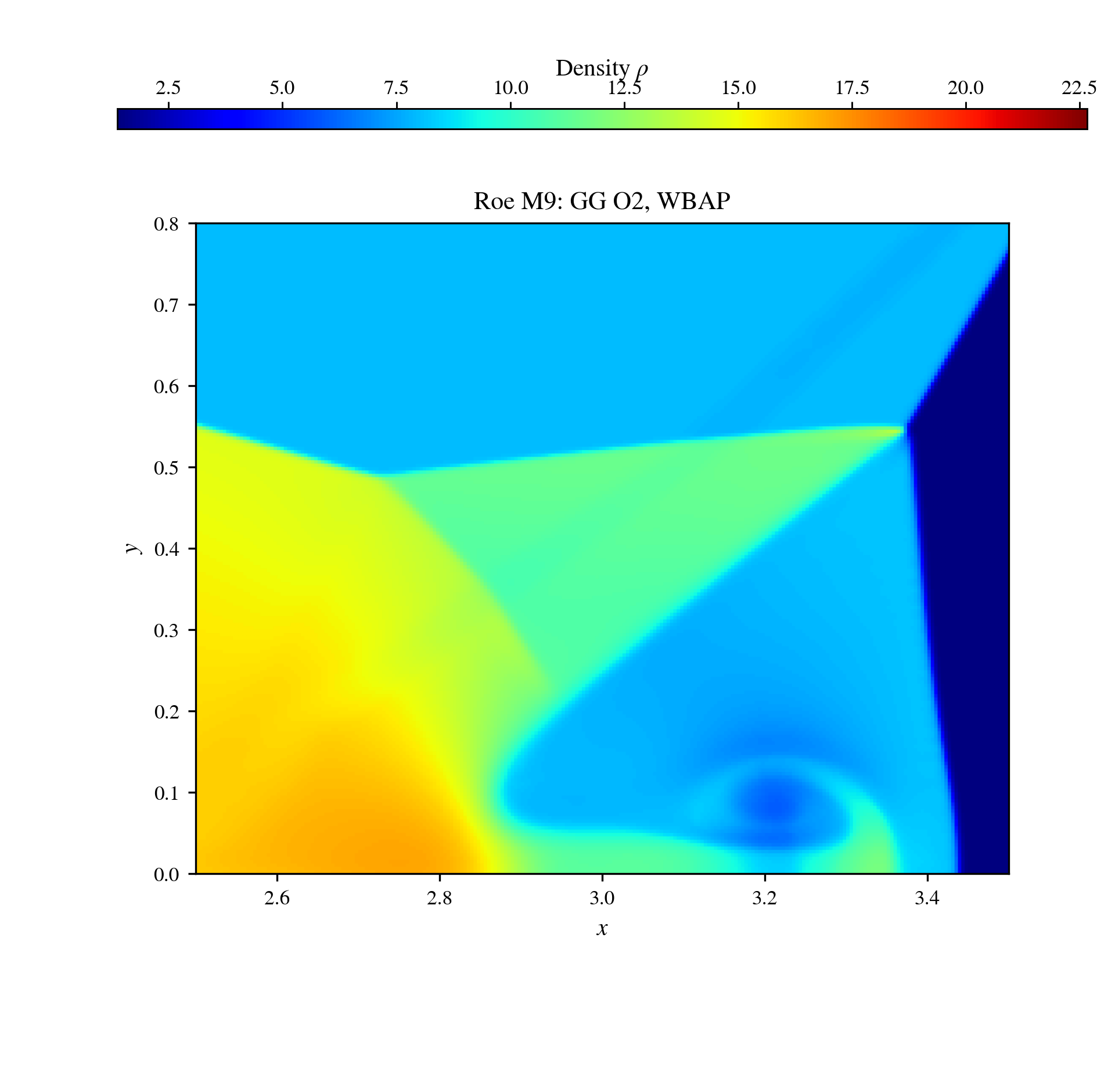
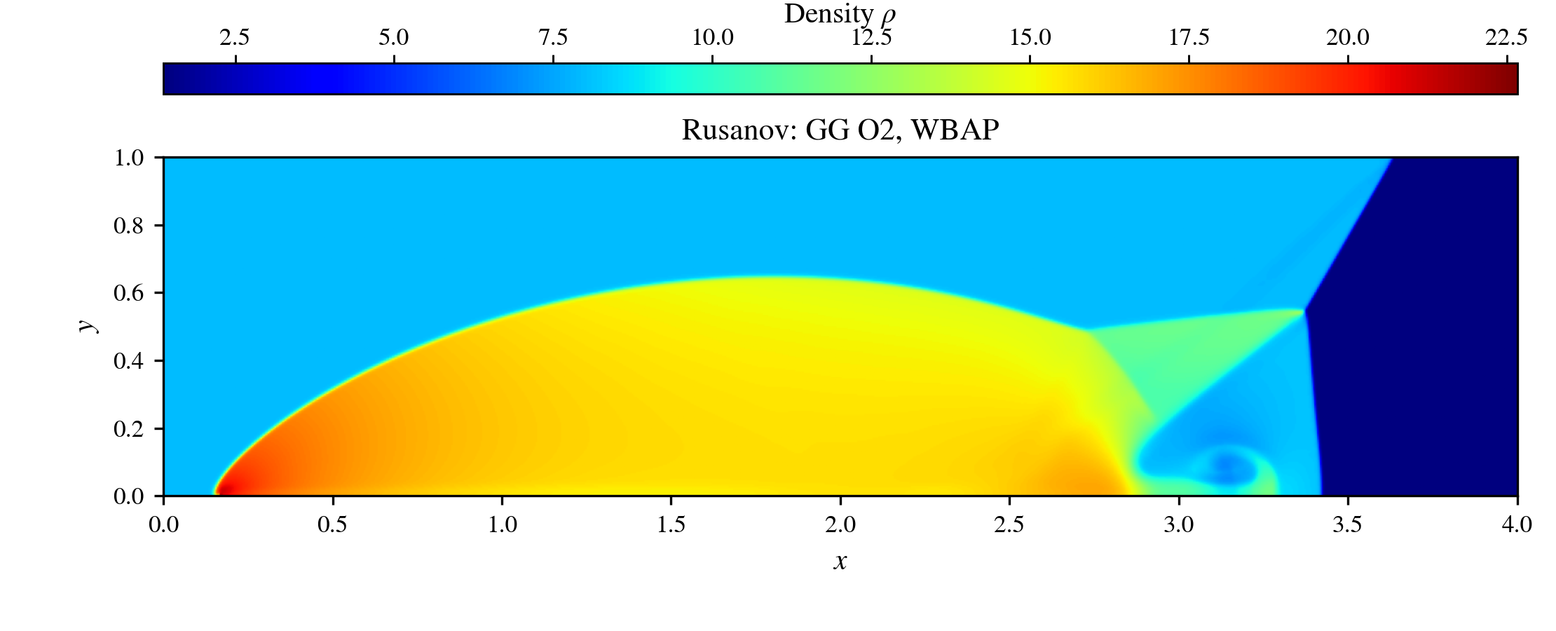
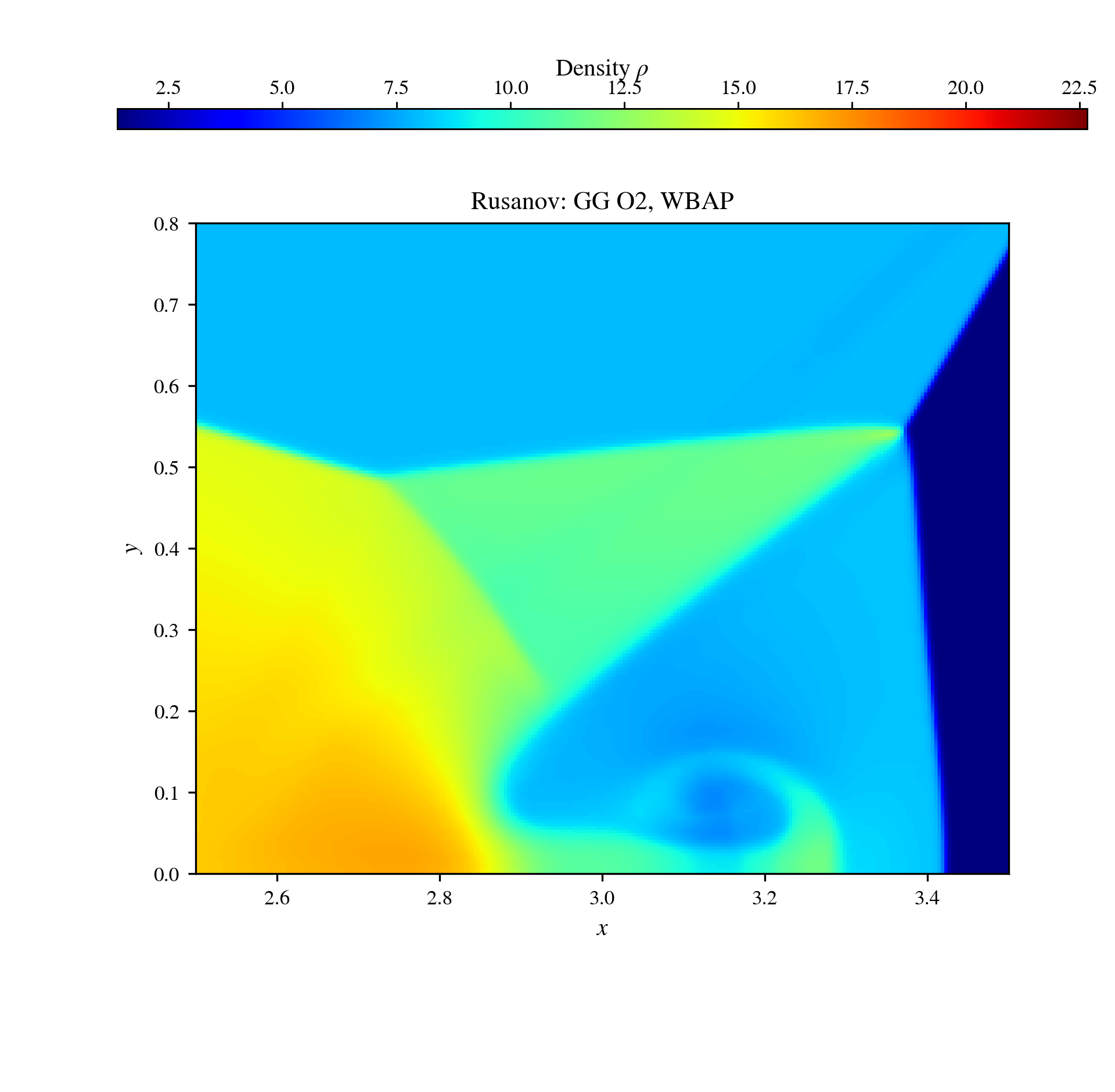
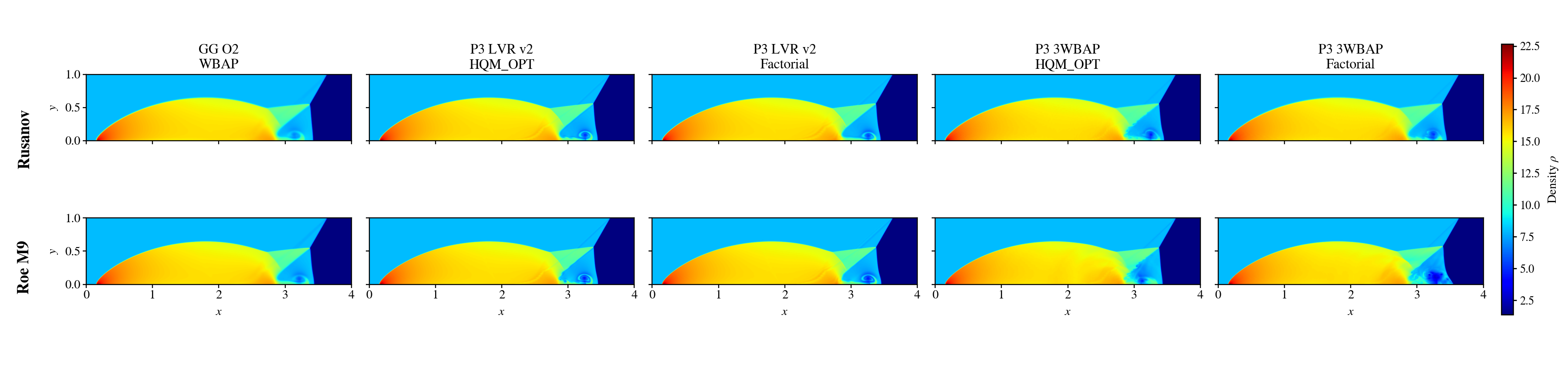
The DMR sequence tests shock geometry, the Mach-reflection triple point, the downstream slip line, wall jet, primary vortex, and Kelvin–Helmholtz roll-up. The triple point is the junction of the incident shock, reflected shock, and Mach stem. The slip line issues downstream from this junction.
Development campaign
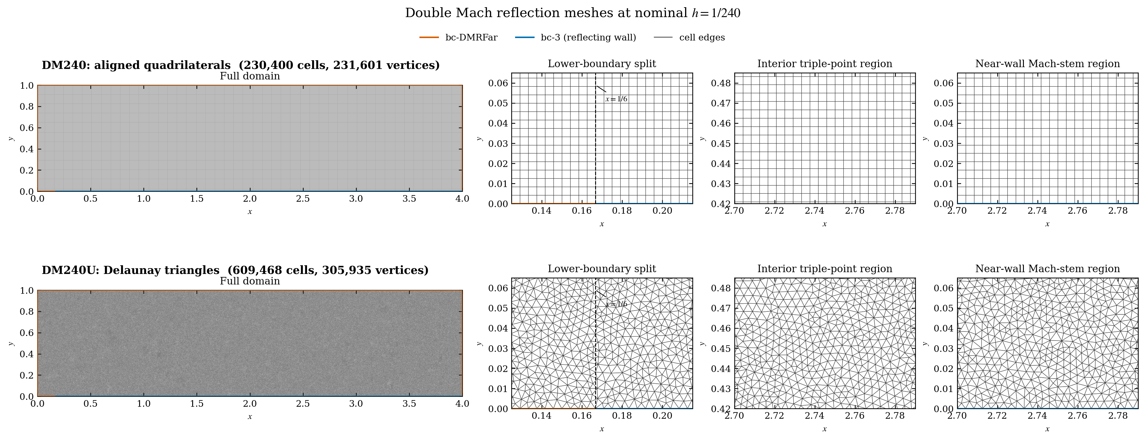
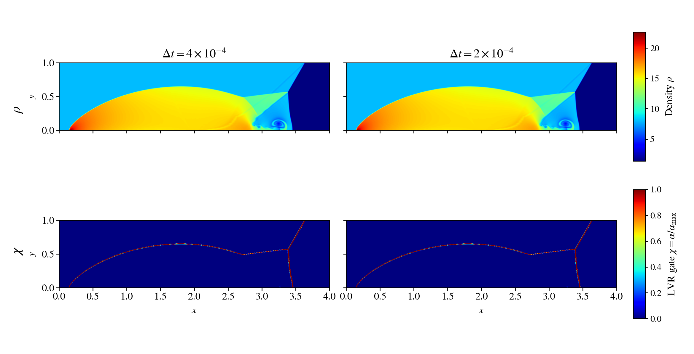
Aligned UniformDM240 contains 230,400 quadrilateral cells. Its Rusanov and Roe M9 sweeps reached $t=0.25$. LVR produces a smooth triple point and delayed slip-line roll-up; halving the time step preserves that result. Fully limited 3WBAP produces more small-scale activity but also a more irregular triple point. The current interpretation is a perturbation-seeding hypothesis: 3WBAP’s irregular shock junction seeds stronger downstream disturbances, whereas LVR leaves the high-order slip line unlimited but supplies it with a quieter initial perturbation.
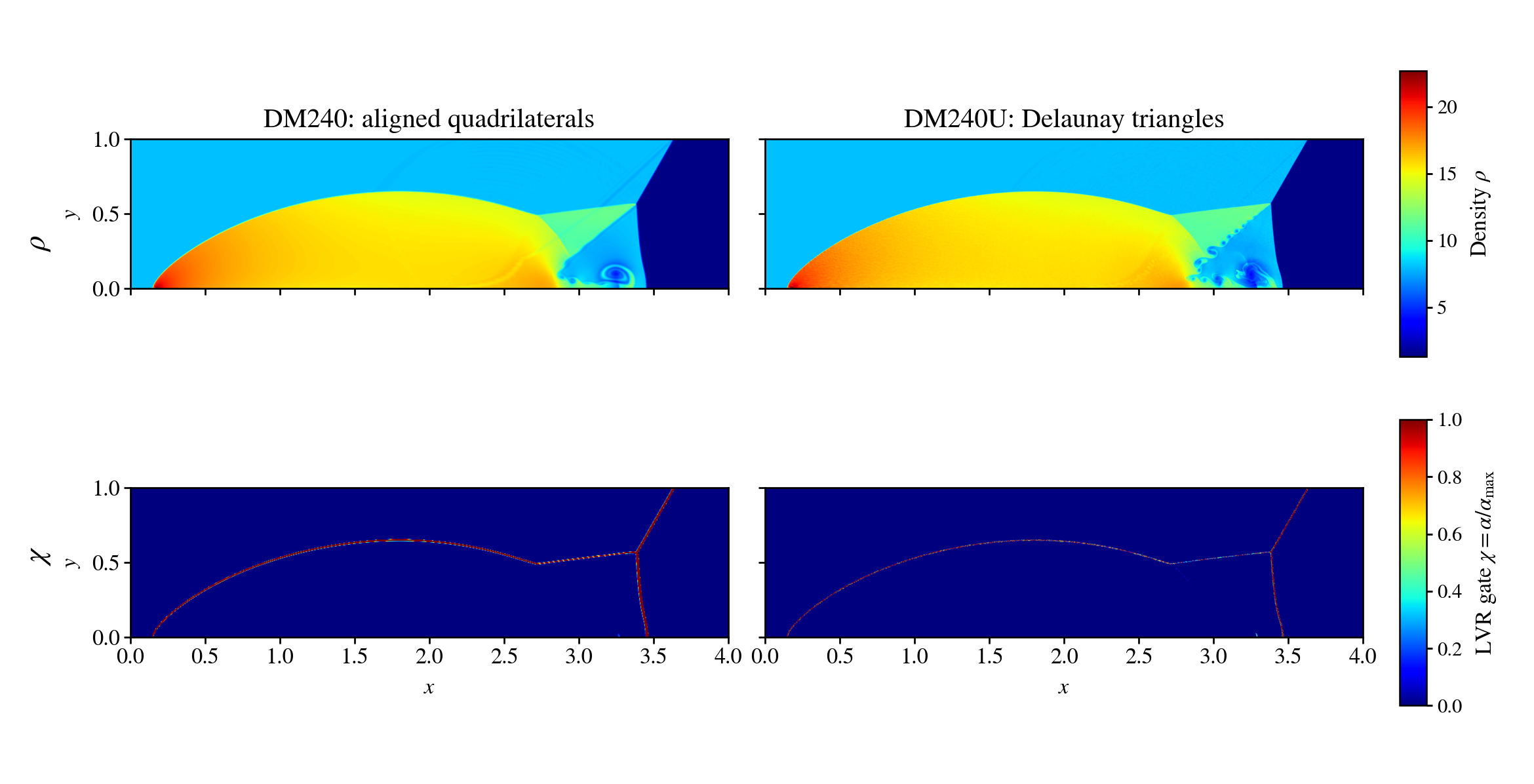
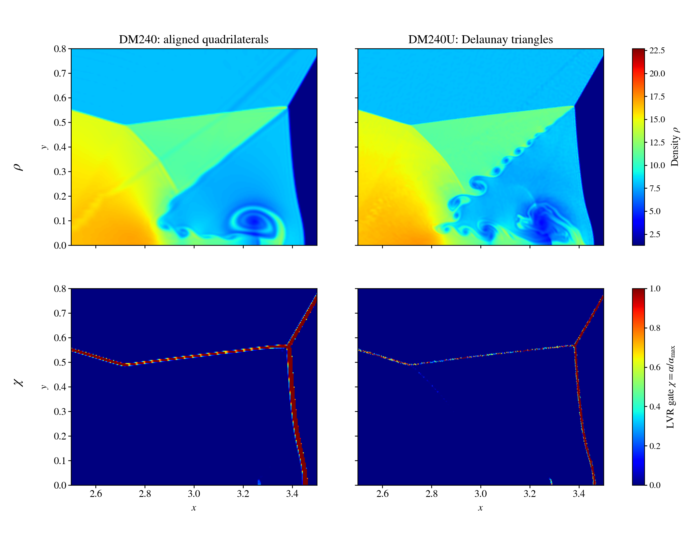
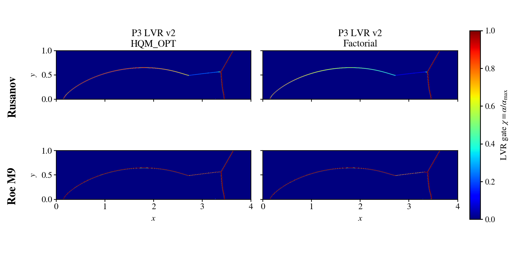
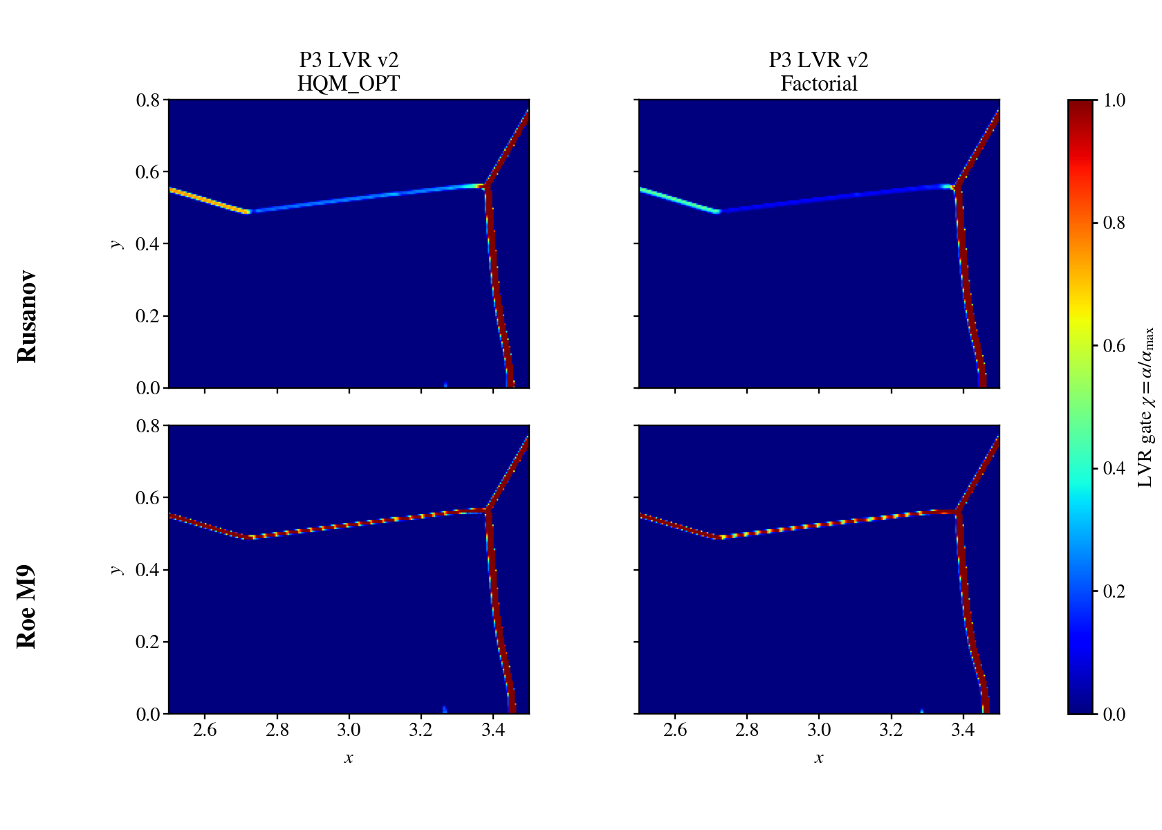
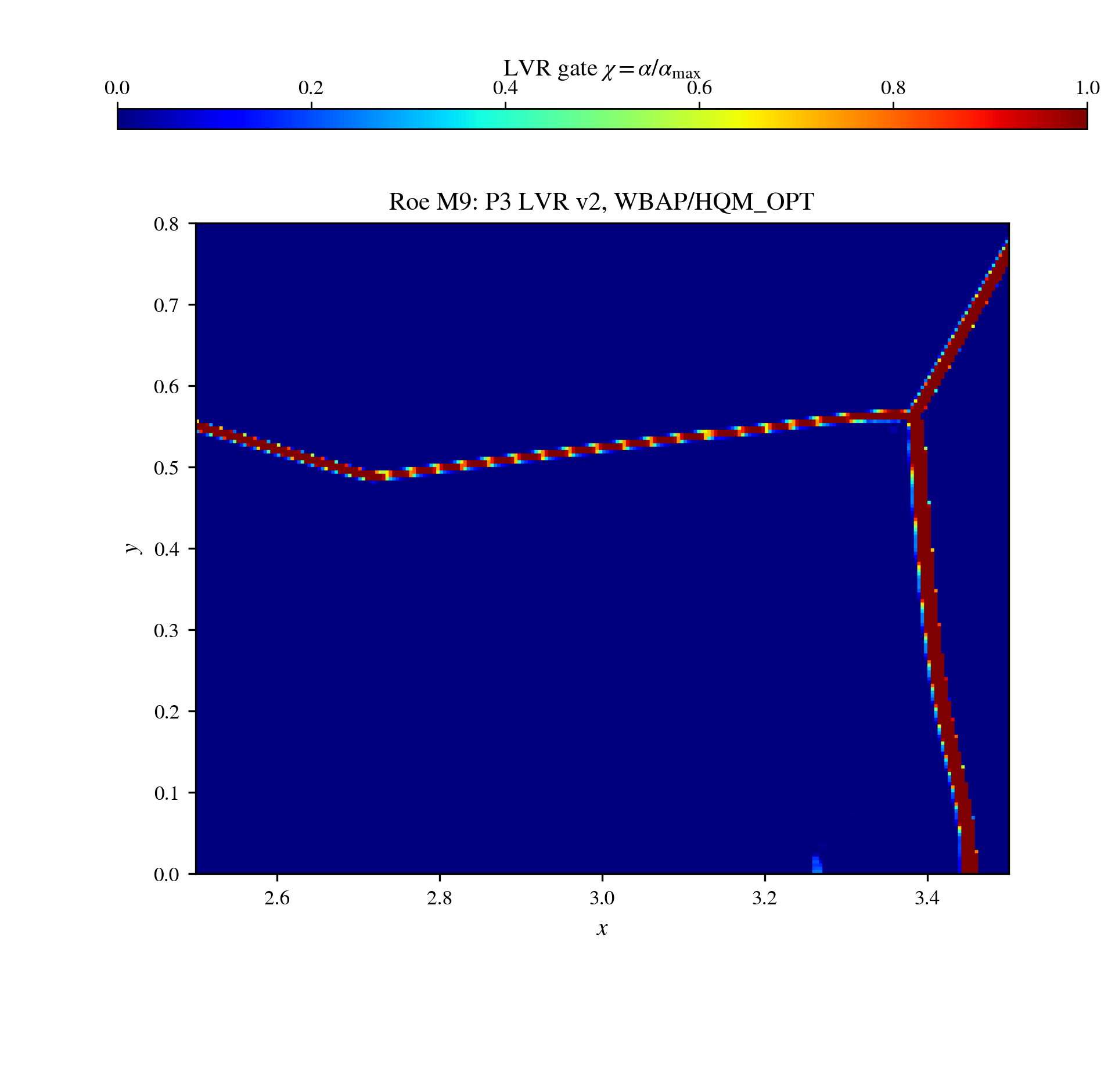
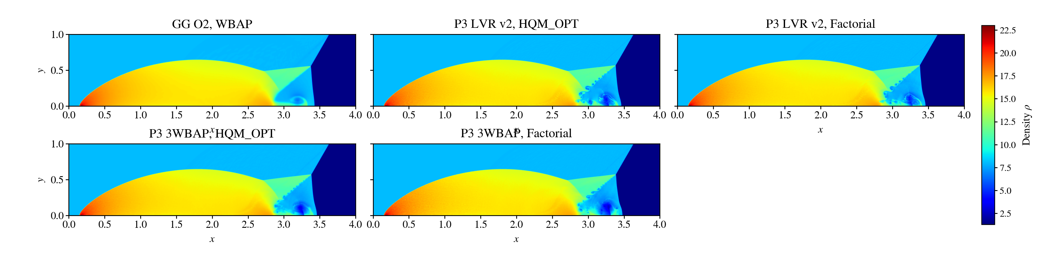
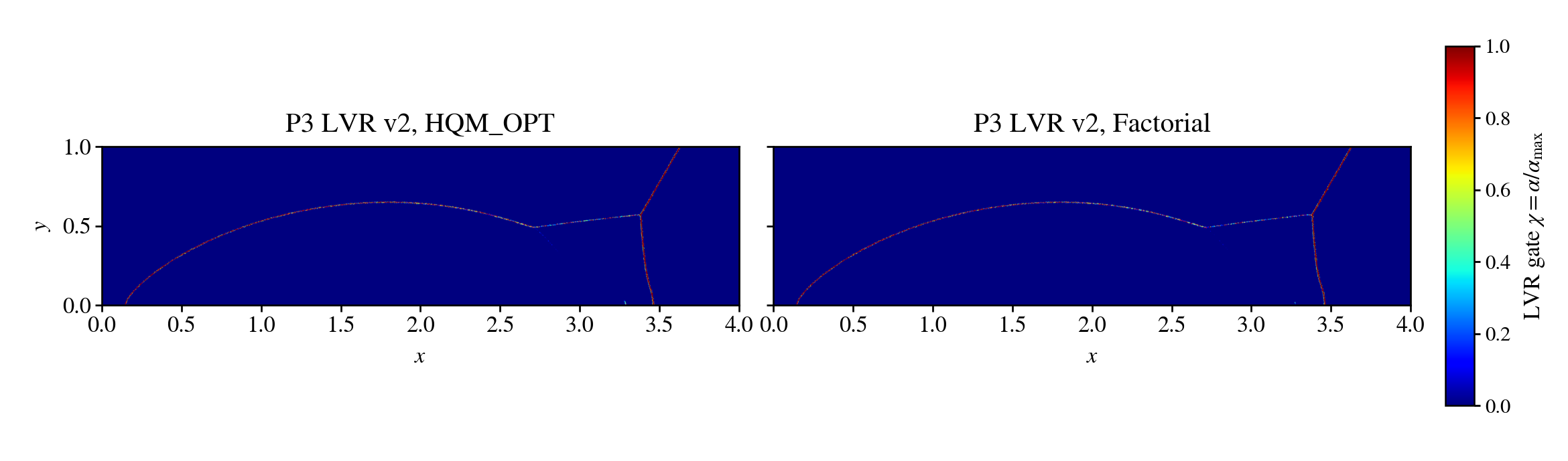
Replacing the aligned mesh with the nominal $h=1/240$ Delaunay DM240U mesh produces 609,468 triangles. Both LVR variants then resolve a long coherent roll-up train while their gate stays concentrated on the shock system. This shows that LVR does not inherently suppress smooth shear-layer instability. The test changes topology, orientation, perturbation spectrum, and cell count, so it does not isolate mesh noise or prove mesh-converged accuracy.
| DM240U method | Wall time | Final density range | Validation |
|---|---|---|---|
| Explicit GG O2/WBAP | 3,028 s | $[1.37913,22.49664]$ | complete |
| LVR v2/HQM_OPT | 11,713 s | $[1.33734,22.46597]$ | reconstructed completion after supervisor loss |
| LVR v2/Factorial | 15,874 s | $[1.33547,22.83554]$ | complete |
| P3 3WBAP/HQM_OPT | 26,148 s | $[1.31685,22.17635]$ | complete |
| P3 3WBAP/Factorial | 27,807 s | $[1.30258,22.00308]$ | complete |
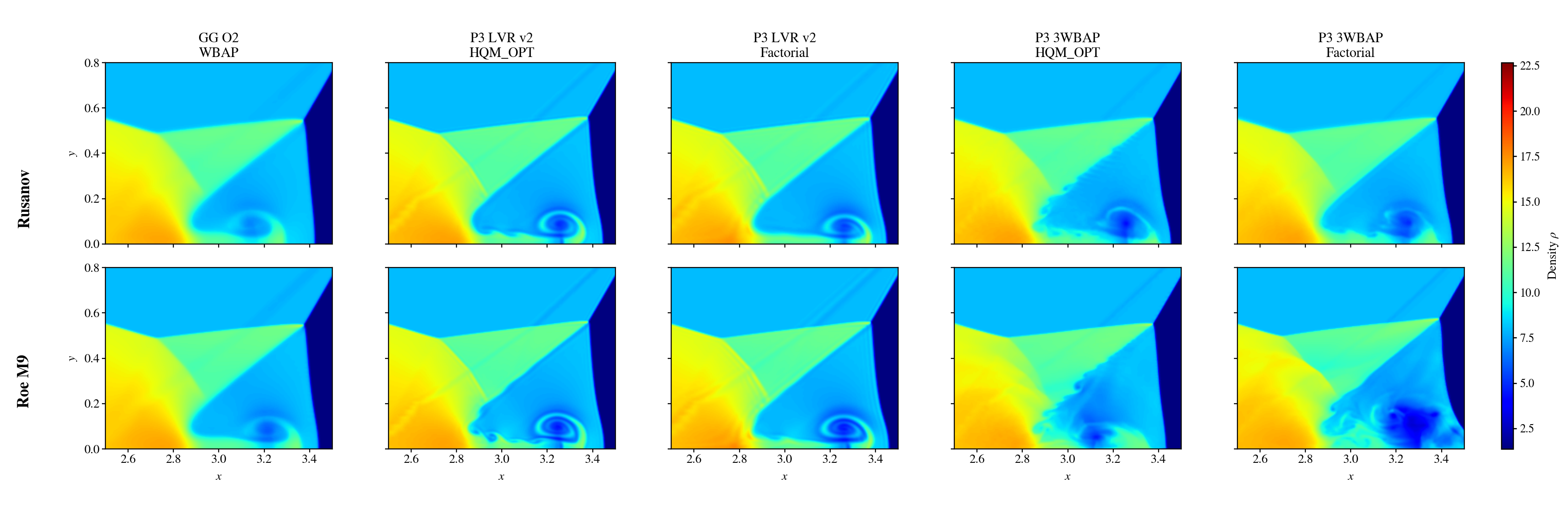
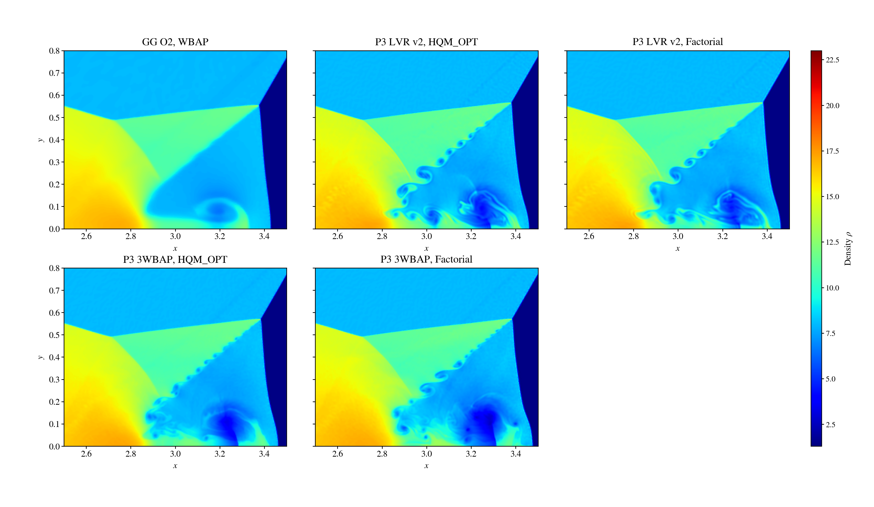
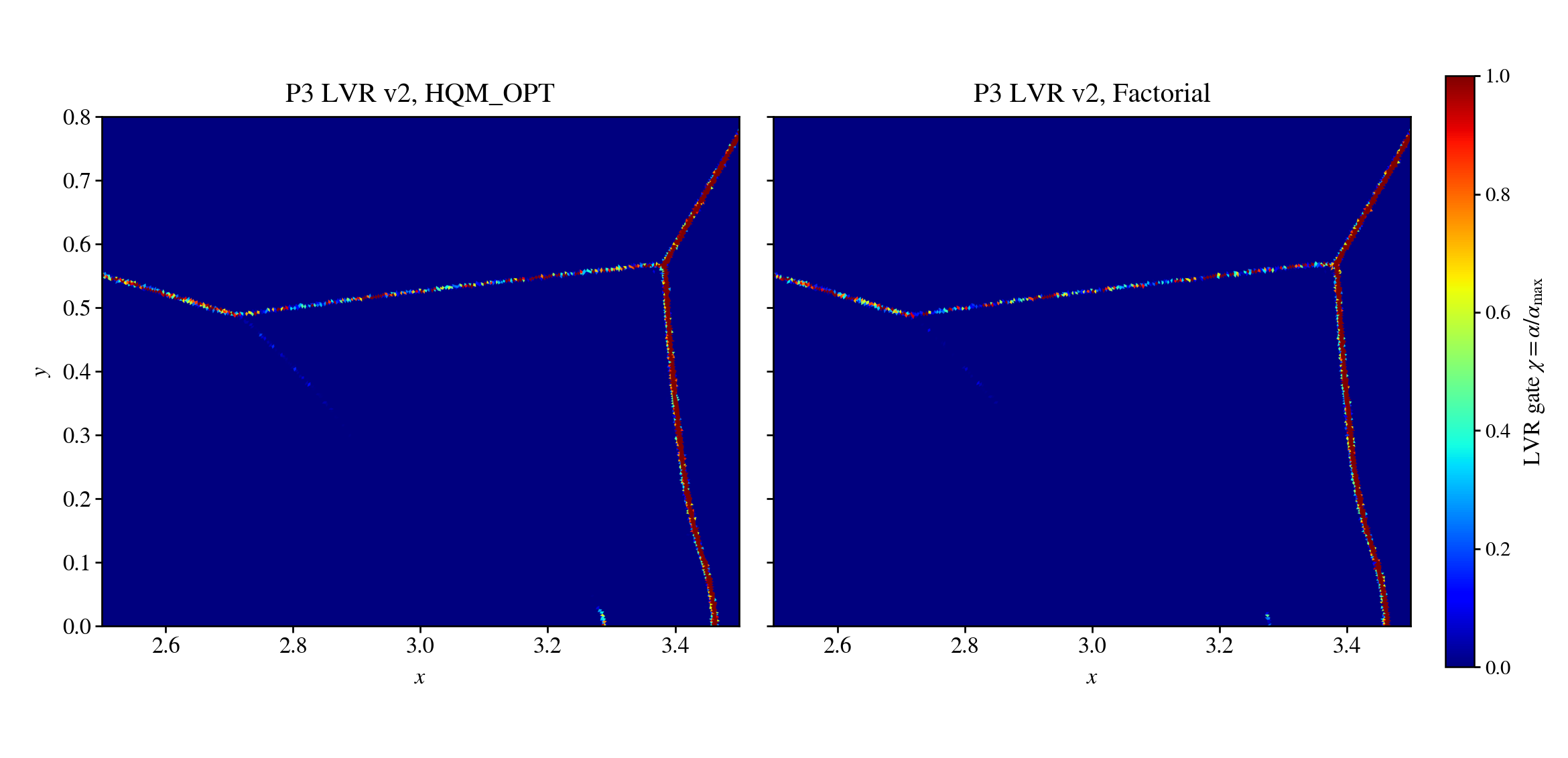
Canonical 13-method DM240U production on thtj1
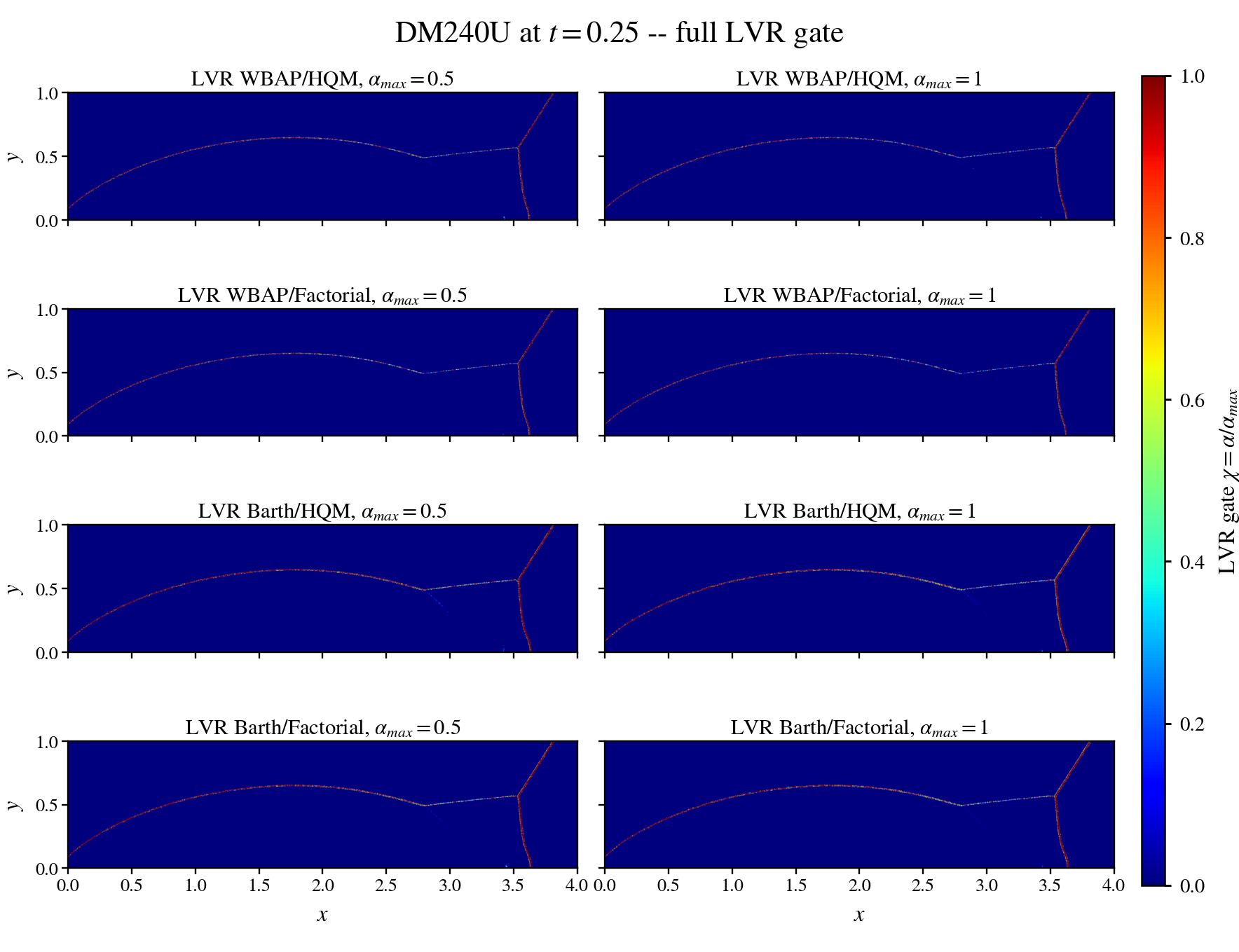
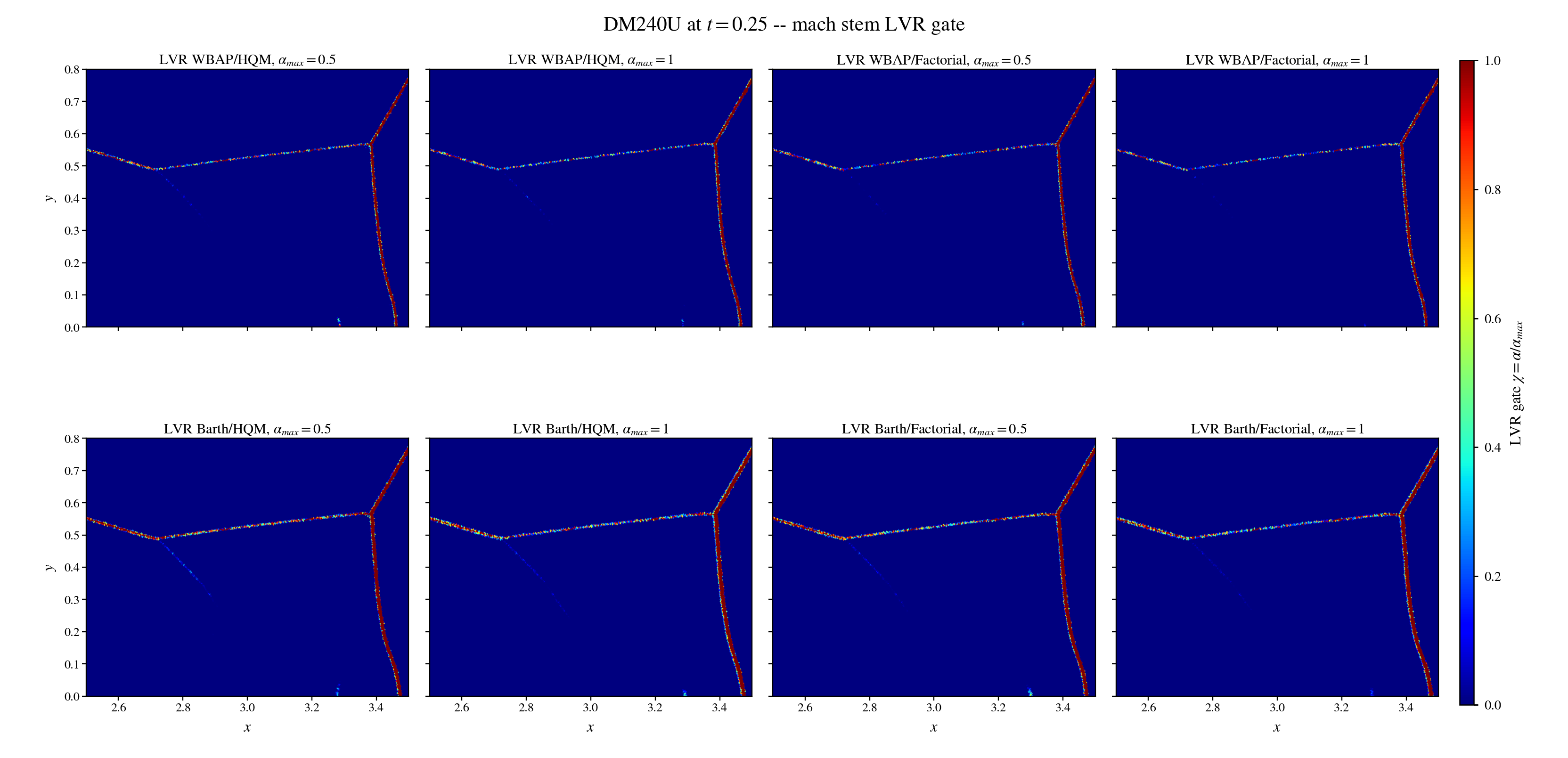
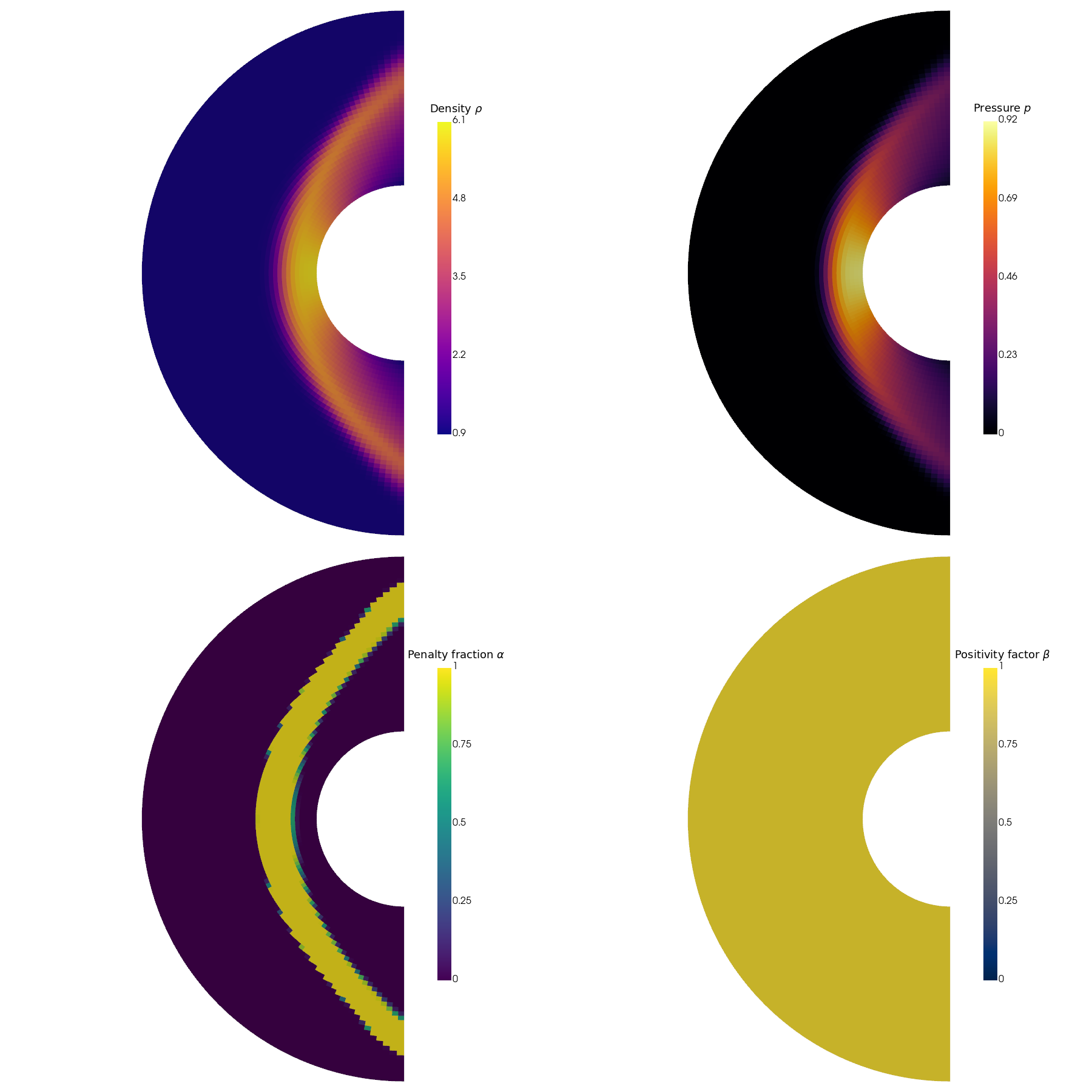
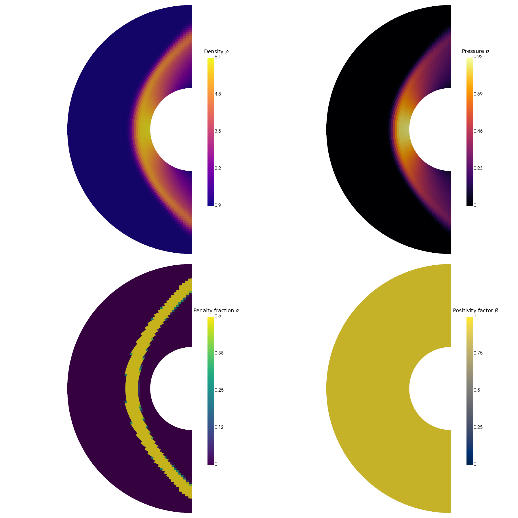
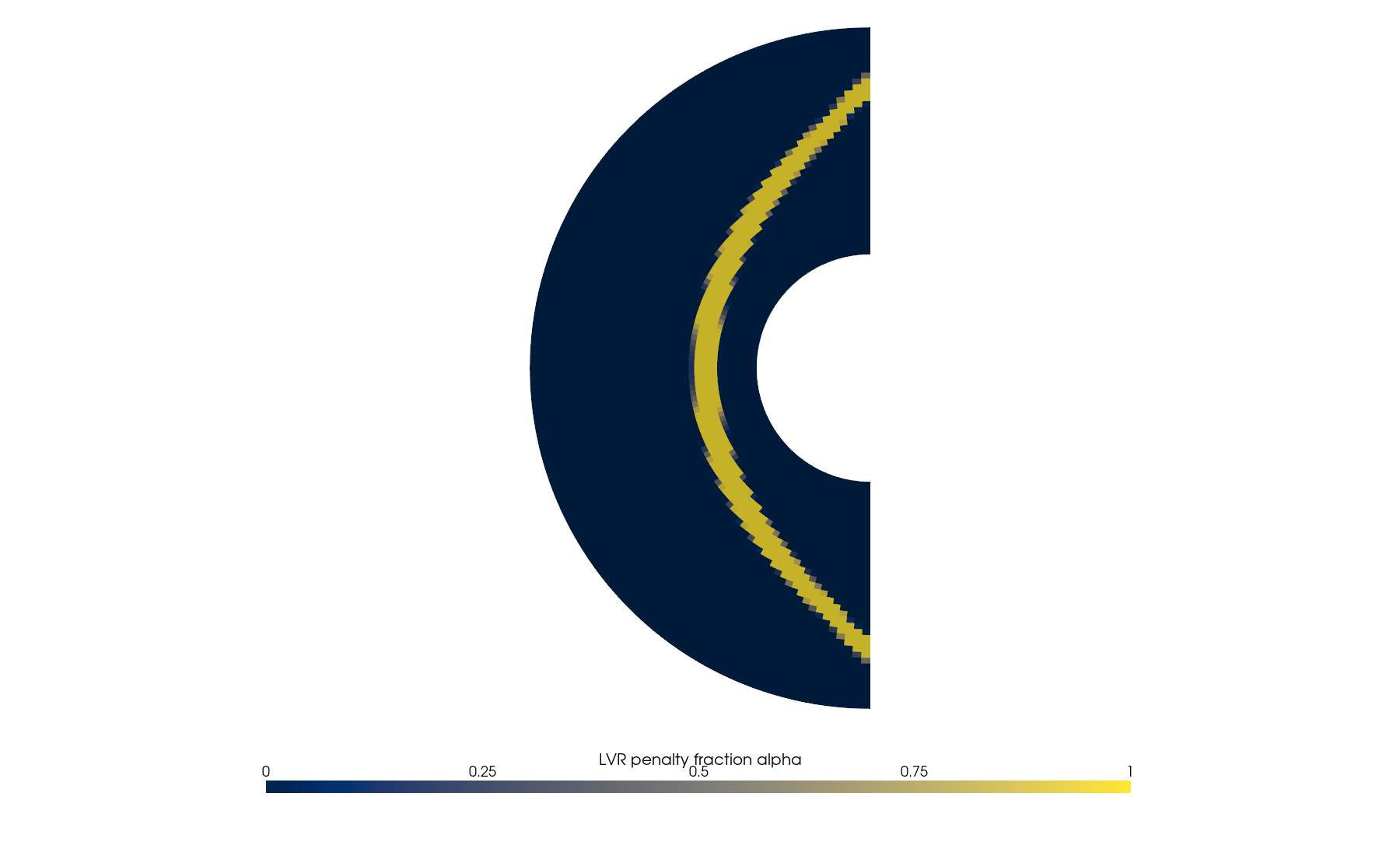
All 13 accepted rows completed on the same 609,468-cell Delaunay mesh with unrotated Roe M9, ESDIRK4, 625 steps of $4\times10^{-4}$ to $t=0.25$, 56 MPI ranks, cell-centered VTKHDF output, and no point output. Final local and remote snapshot hashes agree. The all-method figures use one shared density range $1\le\rho\le24$. The normalized LVR gate is $\chi=\alpha/\alpha_{max}$, so $\chi=0$ is an inactive penalty and $\chi=1$ is the configured maximum penalty.
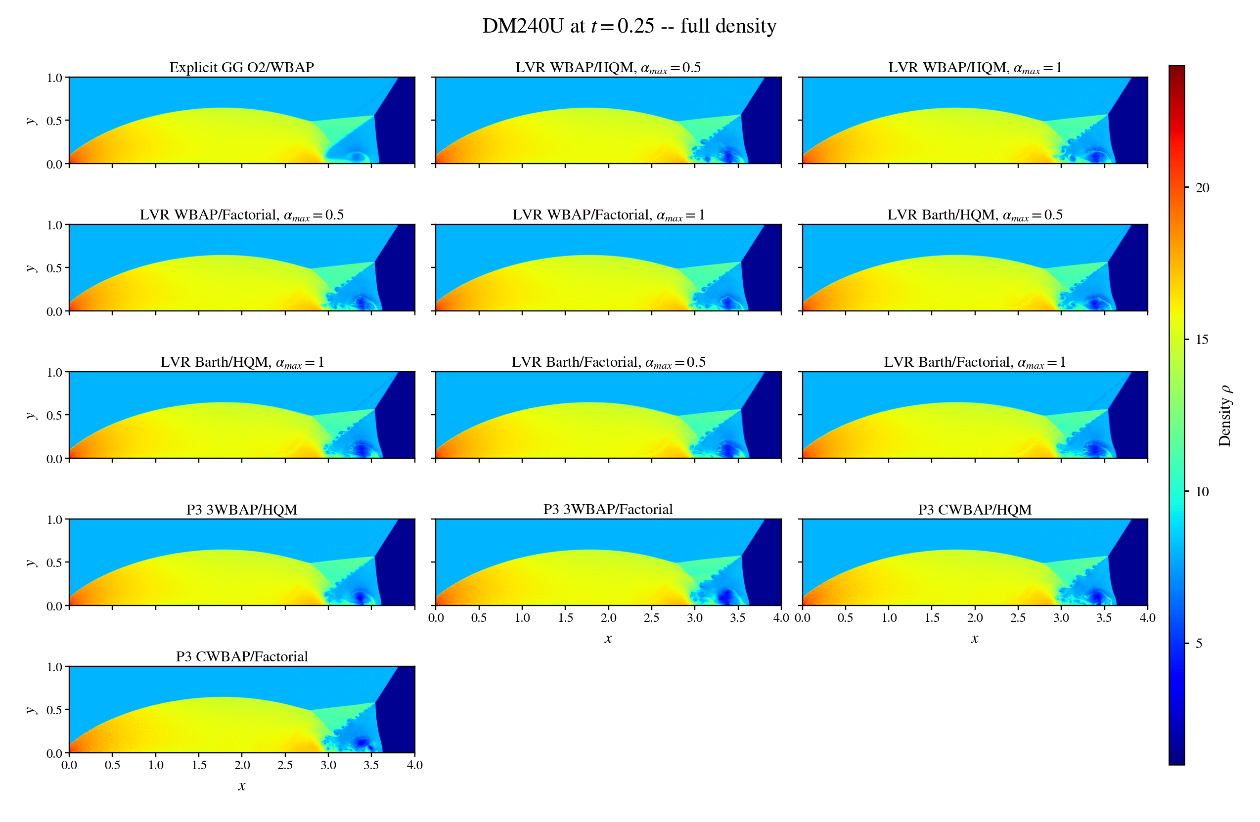
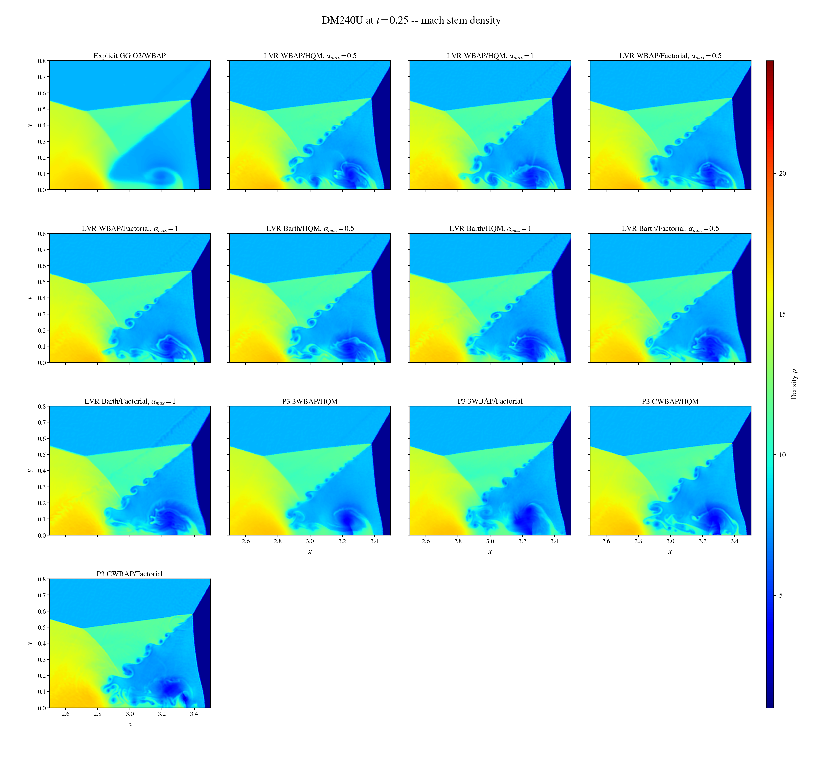
Two-dimensional Riemann problem
Structured 400 x 400 production
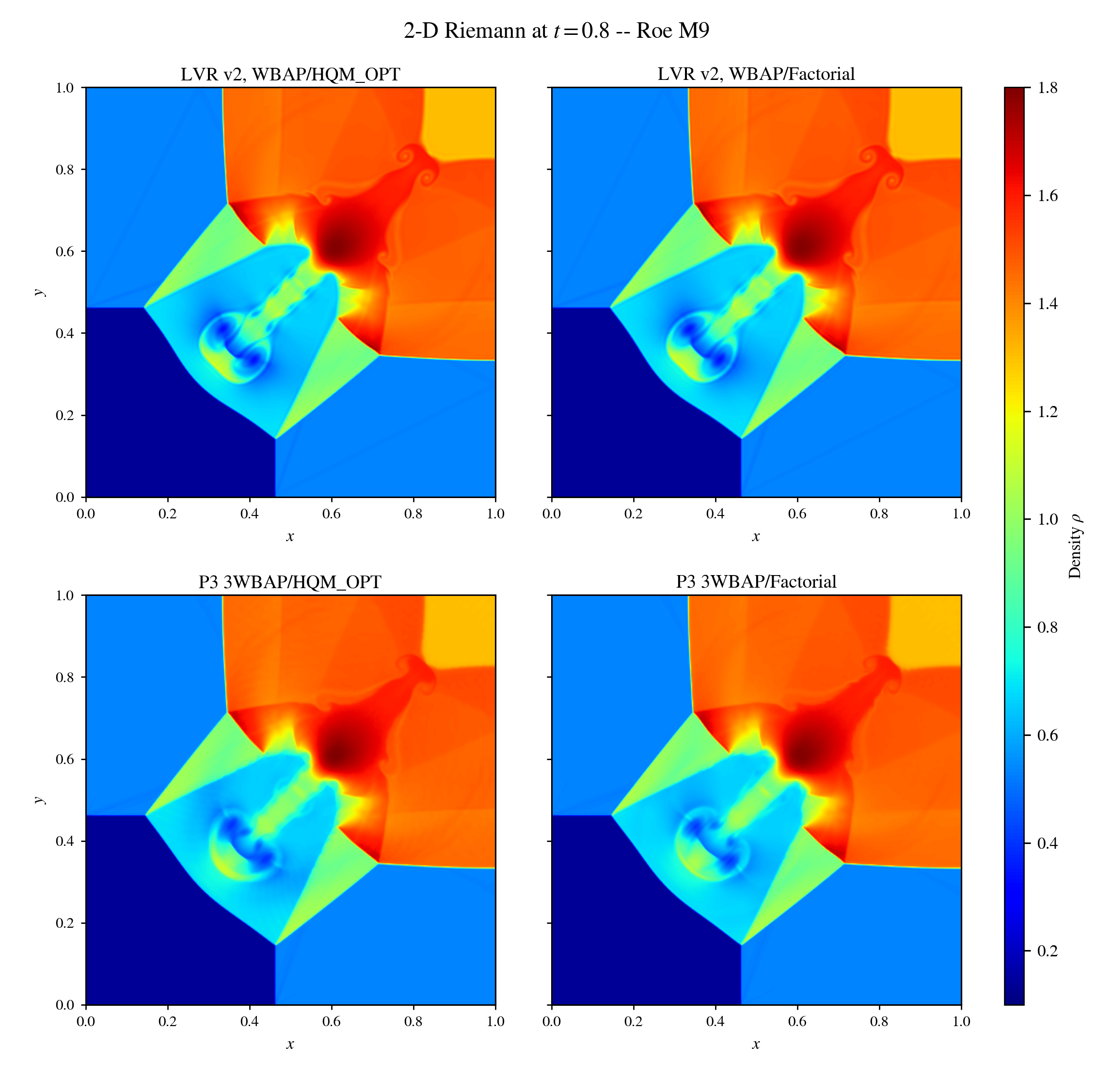
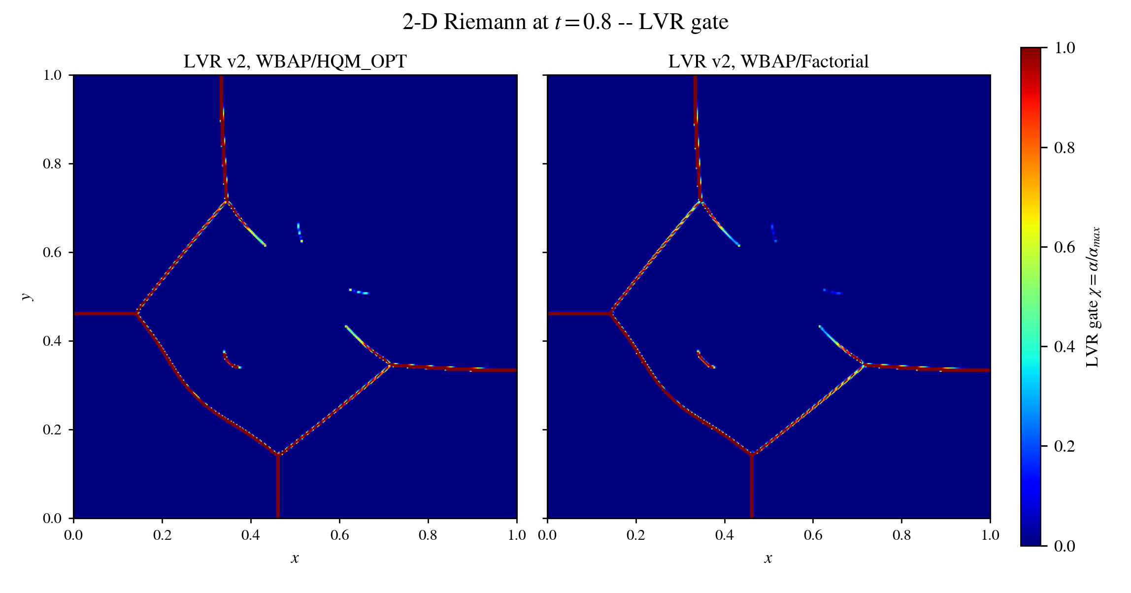
The structured campaign uses 160,000 quadrilateral cells on $[0,1]^2$,
unrotated Roe M9, ESDIRK4, 3,200 steps of $2.5\times10^{-4}$ to $t=0.8$, and
56 MPI ranks on thtj1. Both LVR v2 rows use the WBAP O2 target and
$\alpha_{max}=0.5$; the references are fully limited P3 3WBAP. All four runs
completed with exit code zero, 3,200 final-step markers, finite positive final
states, empty validation-error lists, and nonempty cell-centered VTKHDF
snapshots.
Delaunay 246U production
The unstructured control uses $h=1/246$, 160,420 counterclockwise triangles, 80,703 nodes, and the same domain, initial states, boundary name, flux, time step, final time, and four spatial methods. The cell count differs from the structured reference by only 420 cells.
All four rows completed 3,200 steps at $t=0.8$, returned exit code zero, retained finite positive density and energy, reported no validation errors, and wrote nonempty final cell-centered VTKHDF snapshots. Every snapshot and run record was copied back with matching remote and local SHA-256 hashes.
| Method | Job | State at refresh | Slurm elapsed | Minimum $\rho$ | Minimum $\rho E$ |
|---|---|---|---|---|---|
| LVR v2/WBAP/HQM_OPT | 11790760 | complete | 01:56:23 | 0.120155 | 0.229760 |
| LVR v2/WBAP/Factorial | 11790784 | complete | 01:54:34 | 0.119598 | 0.231224 |
| P3 3WBAP/HQM_OPT | 11790785 | complete | 12:05:34 | 0.125520 | 0.247447 |
| P3 3WBAP/Factorial | 11790786 | complete | 03:59:54 | 0.119668 | 0.236326 |
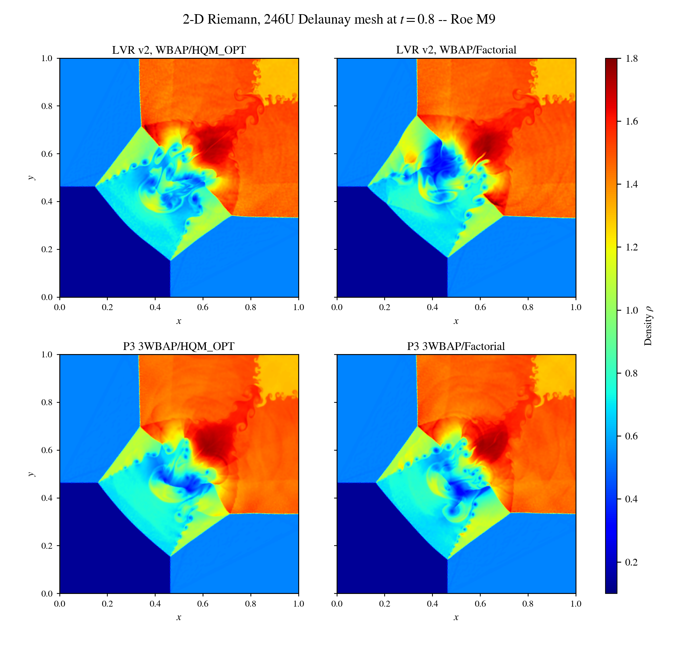
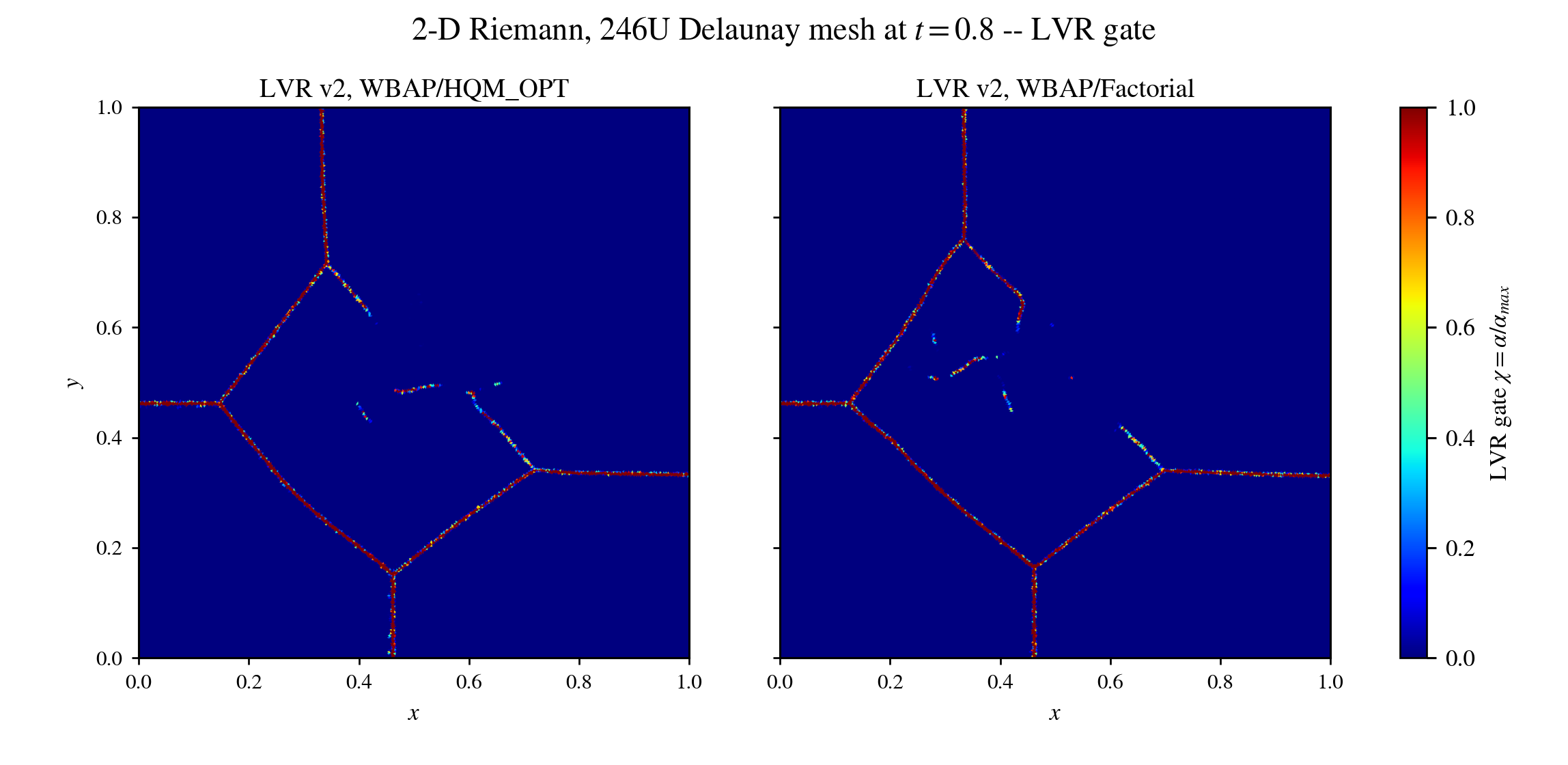
The fixed method order and shared range $0.1\le\rho\le1.8$ make the four final cell-centered density fields directly comparable.
The last completed row can be audited through these remote files on thtj1:
- Slurm output:
/fs2/home/advance/zhy/studies/limited_variational_reconstruction/2026-09-28_riemann2d_400_pilot/slurm_246u/riemann2d-246u-11790785.out - solver standard output:
/fs2/home/advance/zhy/data/lvr/riemann2d_246u_m9_20260928/raw/3wbap_hqm_20260928T154338Z_thtj1-246u-m9-t08_11790785/stdout.log - absolute residual CSV:
/fs2/home/advance/zhy/data/lvr/riemann2d_246u_m9_20260928/raw/3wbap_hqm_20260928T154338Z_thtj1-246u-m9-t08_11790785/riemann2d_.log - run record:
/fs2/home/advance/zhy/studies/limited_variational_reconstruction/2026-09-28_riemann2d_400_pilot/records/3wbap_hqm_20260928T154338Z_thtj1-246u-m9-t08_11790785.json
Main findings
- The $\mathbf A_i$-weighted penalty is algebraically compatible with the existing block Jacobi/GS/SOR machinery. It produces an exact convex target without rebuilding the cached cell inverse.
- A characteristic WBAP-limited O2 target is materially better than the Barth target for the selected strong-shock comparisons, although the Barth path remains useful as an ablation.
- The original pressure-jump/compression product gate localizes shocks and avoids pure expansions and shear layers, but its two indicators can be spatially offset beside a strong shock.
- LVR v2’s shock-supported extremum correction closes that Lax gate gap and reduces the shoulder oscillation by about 94% without changing the curved cylinder bow-shock solution.
- LVR v2 preserves convergence advantages over fully limited high-order schemes in the steady cylinder and is consistently much cheaper than fully limited 3WBAP in the current multidimensional runs.
- The DMR results show that a quiet LVR triple point can delay slip-line roll-up, while the unstructured-mesh control shows that LVR still resolves substantial Kelvin–Helmholtz structure when perturbations are supplied by the mesh. Vortex count alone is not an accuracy metric.
- The structured and completed unstructured 2-D Riemann contours show that the derivative-weight choice changes the developed interaction substantially, even when the LVR gate remains concentrated on discontinuities.
Limitations and next steps
- Replace the equal-pressure-neighbour count with a geometric tangential smoothness test based on the limited-O2 pressure-gradient direction. This is needed for a mesh-independent multidimensional v2 gate.
- Repeat Lax and multidimensional cases on refinement sequences to measure the physical width of the corrected band and verify that plateau flatness is not tied to the current spacing.
- Repeat the structured and Delaunay 2-D Riemann comparisons on a refinement sequence to separate derivative-weight sensitivity from mesh-scale effects.
- Separate DMR perturbation seeding from dissipation using matched degrees of freedom, time-resolved slip-line growth, and one common imposed disturbance.
- Retain the Toro 123 positivity failure as a hard screen for Roe variants; gate widening must not be accepted by shock-tube appearance alone.
- For Shu–Osher, assess post-shock phase, amplitude, $L_1/L_2$, total variation, and gate overlays together.
Complete figure atlas
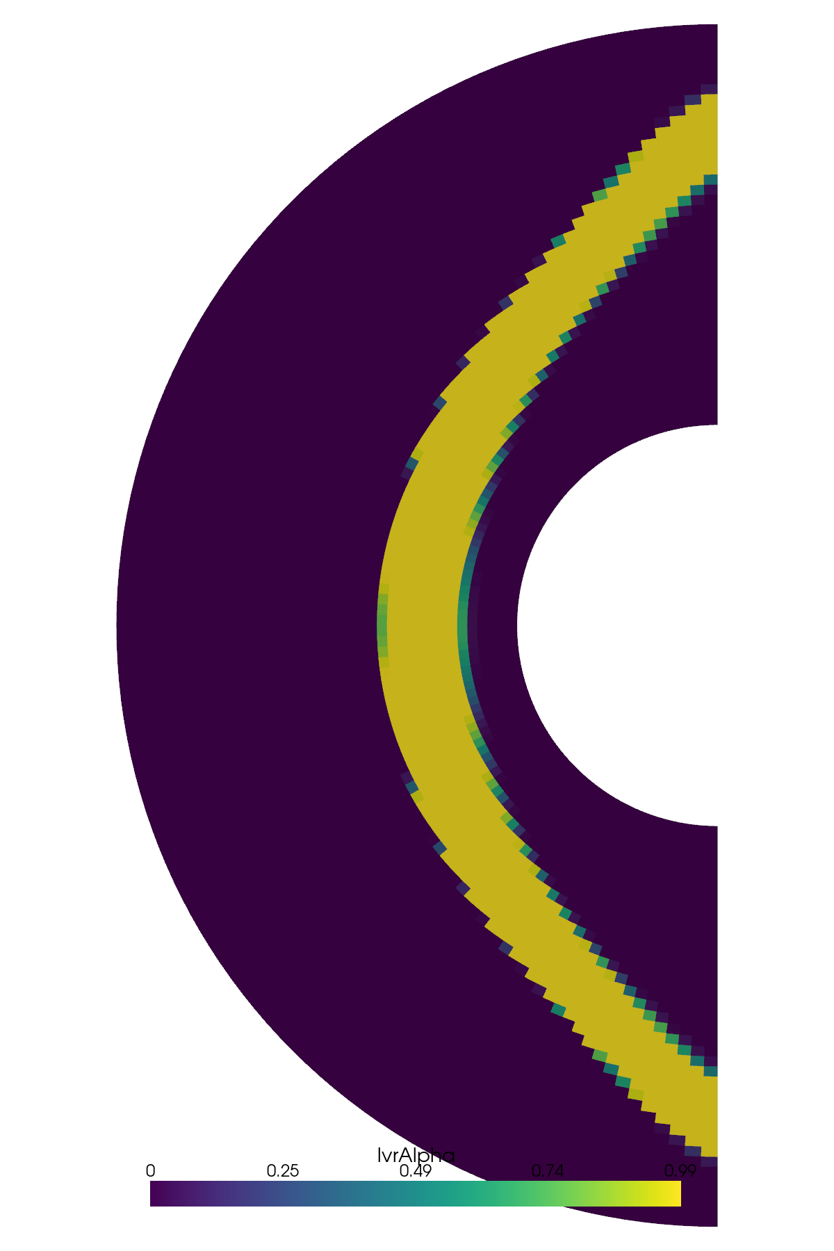
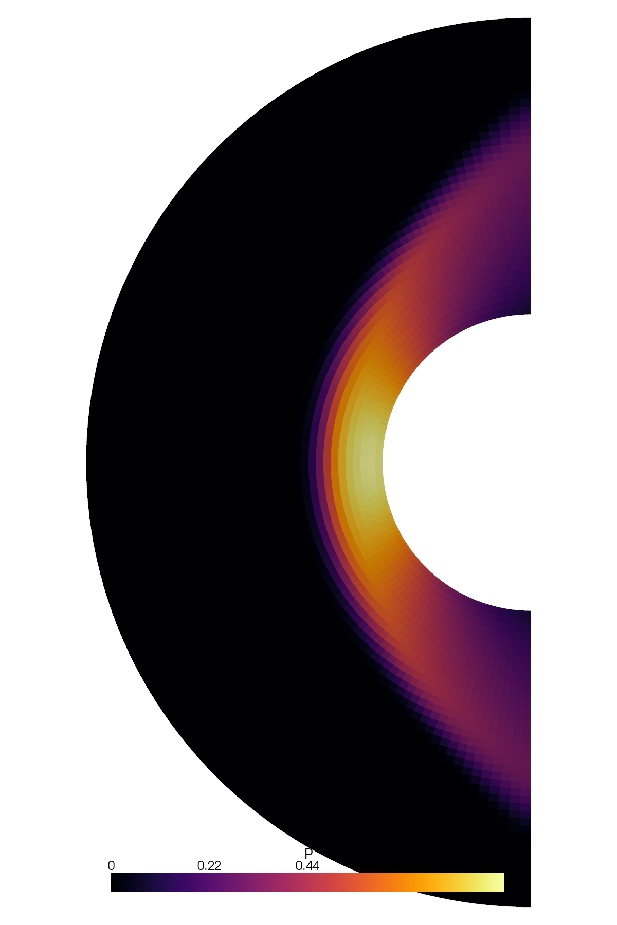
The atlas below embeds every top-level PNG generated by the studies used in this post. It intentionally excludes duplicate PDFs and internal rendering tiles.
Initial method validation (10 figures)
| Figure | Figure |
|---|---|
 |  |
 |  |
 |  |
 |  |
 |  |
Initial parameter tuning (2 figures)
| Figure | Figure |
|---|---|
 |  |
Uniform-start cylinder convergence (1 figure)
| Figure | Figure |
|---|---|
 |
WBAP O2 reference retuning (7 figures)
| Figure | Figure |
|---|---|
 |  |
 |  |
 |  |
 |
HQM_OPT joint tuning (5 figures)
| Figure | Figure |
|---|---|
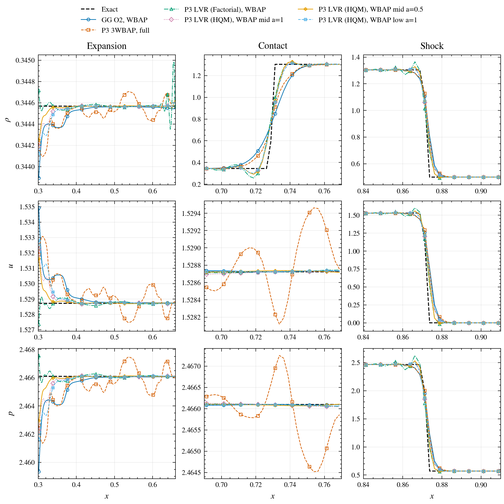
 |  |
 | 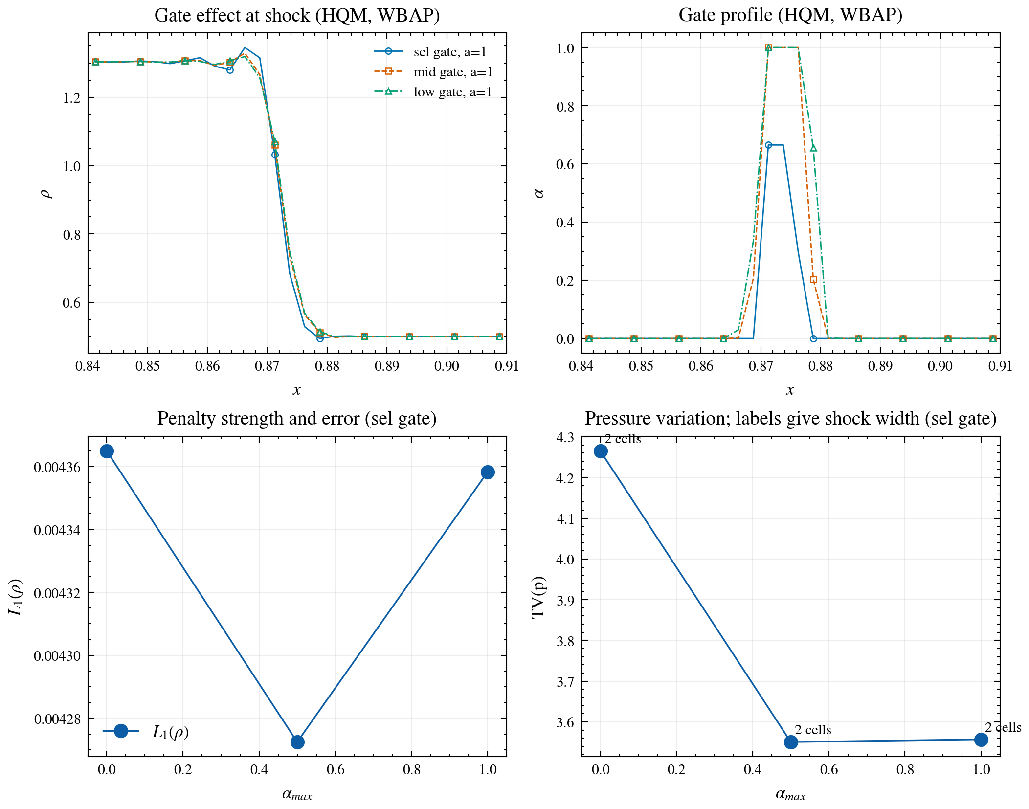 |
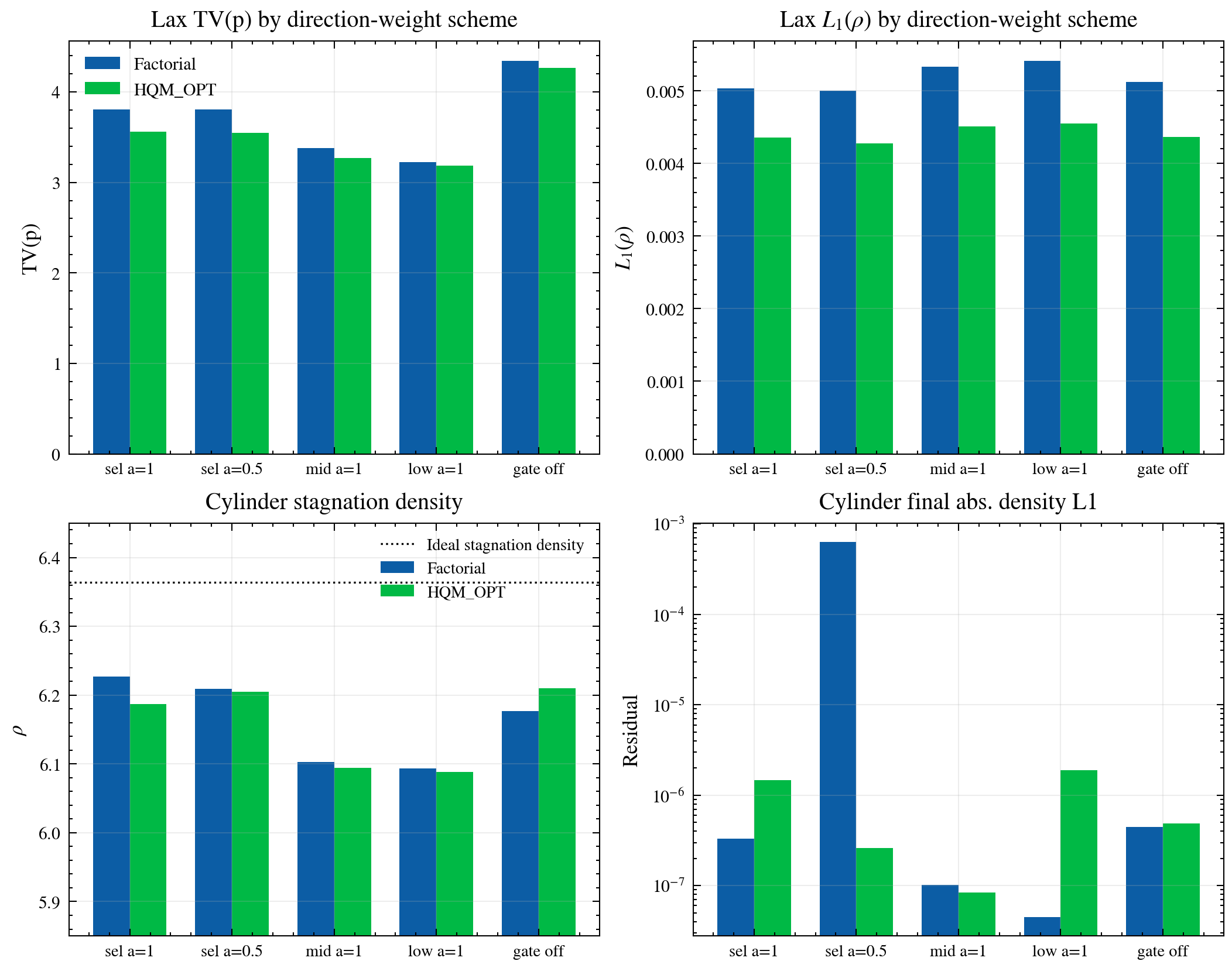 |
LVR v2 shock-band gate (3 figures)
| Figure | Figure |
|---|---|
| |
|
LVR v2 extended validation (13 figures)
| Figure | Figure |
|---|---|
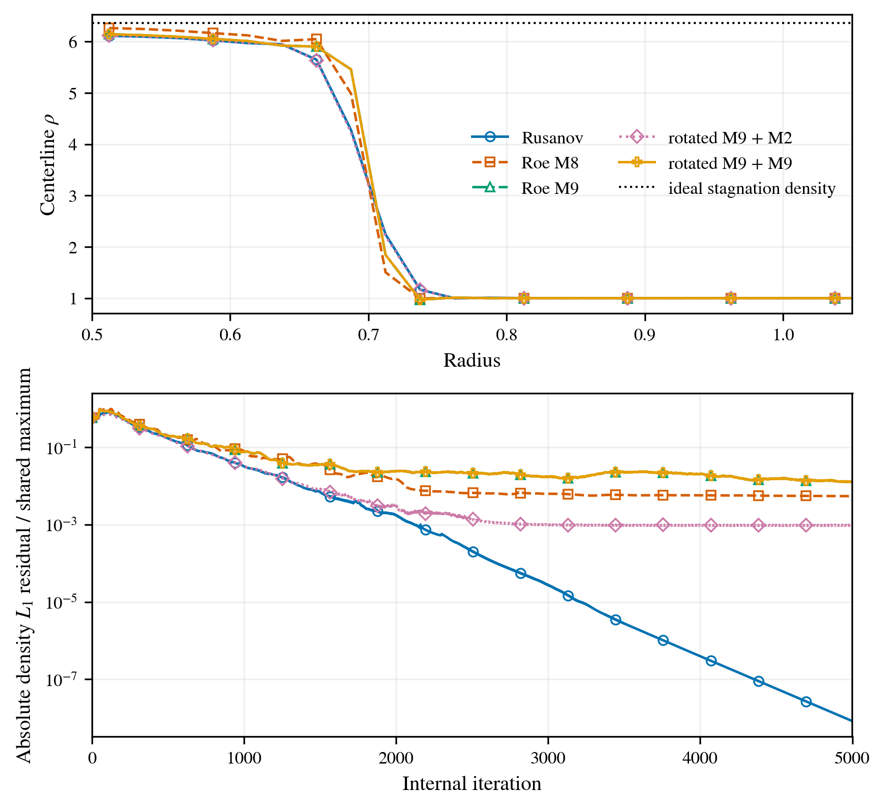 |  |
|  |
 | |
 |  |
 |  |
 |  |
 |
Double Mach reflection development (41 figures)
| Figure | Figure |
|---|---|
 |  |
 |  |
 |  |
 |  |
 |  |
 |  |
 |  |
 |  |
 |  |
 |  |
 |  |
 |  |
 |  |
 |  |
 |  |
 |  |
 |  |
 |  |
|  |
|  |
|
Canonical 13-method matrix (30 figures)
| Figure | Figure |
|---|---|
| |
| |
| |
| |
| |
| |
| |
| |
| |
| |
| |
| |
| |
| |
| |
Two-dimensional Riemann campaigns (4 figures)
| Figure | Figure |
|---|---|
| |
| |