MG-FAS
非线性问题
- 非线性问题:
- 牛顿迭代:
- 近似+松弛的牛顿迭代:
- 松弛迭代(非线性):
- 逐点更新$𝑥_𝑖$(可同时更新$𝐹_𝑖$,如非线性GS)
- 牛顿迭代可以视作一种特殊的松弛
- 牛顿迭代内部采用不同的线性求解器,也可以是松弛迭代
FAS中,计算\(∆𝑥\)更新求解本级的\(𝐹(𝑥)=0\),即为一个松弛步/光滑步。
FAS 通用过程
- Relax:通过密网格残差 $𝐹^ℎ (𝑥^{ℎ,𝑚})$ 计算 $𝑦^{ℎ,𝑚}=𝑥^{ℎ,𝑚}+∆𝑦^{ℎ,𝑚}$
- Restrict:$𝑦^{2ℎ,𝑚}=𝐼_ℎ^{2ℎ} 𝑦^{ℎ,𝑚}$, $𝑟^{2ℎ}=𝐼_ℎ^{2ℎ} 𝐹^ℎ (𝑦^{ℎ,𝑚})$
- Relax: 2h网格上的待解方程:$𝐹^{2ℎ} (𝑥^{2ℎ} )=𝐹^{2ℎ} (𝑦^{2ℎ,𝑚} )−𝑟^{2ℎ}$
- 其中初值即为$𝑥^{2ℎ,0}=𝑦^{2ℎ,𝑚}$
- 求解后得到$𝑥^{2ℎ,𝑙𝑎𝑠𝑡}=𝑥^{2ℎ,0}+𝑒^{2ℎ, 𝑚}$
- Interpolate: $𝑒^{ℎ, 𝑚}=𝐼_{2ℎ}^ℎ 𝑒^{2ℎ, 𝑚}$, $𝑥^{ℎ,𝑚+1}=𝑦^{ℎ,𝑚}+𝑒^{ℎ, 𝑚}$
此处的$F^{2h}$为疏网格的算子。
投影/限制算子:$𝐼_ℎ^{2ℎ}$ 与 插值算子: $𝐼_{2ℎ}^ℎ$ 为线性算子。
以上$h,2h$为一相对概念,代表两级网格间的操作关系;$h,2h$仅为符号,对应的不一定是网格尺度2倍,可能是代数MG算子,或者非结构网格的几何融合,也可能是谱空间截断/多项式投影等不同解空间。
针对双时间步的说明:
$$ F(x)=\alpha R(x) - \frac{x}{\Delta t} + B $$其中 $R(x)=\dv{x}{t}, \alpha > 0$
两级网格间的操作:
- Relax:通过密网格残差 $$ \widehat{𝐹}^ℎ (𝑥^{ℎ,𝑚}) = \alpha R^{h}(x^{ℎ,𝑚}) - \frac{x^{ℎ,𝑚}}{\Delta t} + B^{h} $$ 计算 $𝑦^{ℎ,𝑚}=𝑥^{ℎ,𝑚}+∆𝑦^{ℎ,𝑚}$
- Restrict:$𝑦^{2ℎ,𝑚}=𝐼_ℎ^{2ℎ} 𝑦^{ℎ,𝑚}$ $$ B^{2h}=𝐼_ℎ^{2ℎ}\alpha R^h(𝑦^{ℎ,𝑚}) + 𝐼_ℎ^{2ℎ} B^h - \alpha R^{2h}(𝑦^{2ℎ,𝑚}) $$
- Relax: 2h网格上的待解方程:
$$
\widehat{𝐹}^{2ℎ} (𝑥^{2ℎ}) = \alpha R^{2h}(𝑥^{2ℎ}) - \frac{𝑥^{2ℎ}}{\Delta t} + B^{2h}
$$
- 其中初值即为$𝑥^{2ℎ,0}=𝑦^{2ℎ,𝑚}$
- 求解后得到$𝑥^{2ℎ,𝑙𝑎𝑠𝑡}=𝑥^{2ℎ,0}+𝑒^{2ℎ, 𝑚}$
- Remark: 若 $\widehat{𝐹}^ℎ (y^{ℎ,𝑚})=0$,则有$\widehat{𝐹}^{2ℎ} (y^{2ℎ,𝑚})=0$
- Interpolate: $𝑒^{ℎ, 𝑚}=𝐼_{2ℎ}^ℎ 𝑒^{2ℎ, 𝑚}$, $𝑥^{ℎ,𝑚+1}=𝑦^{ℎ,𝑚}+𝑒^{ℎ, 𝑚}$
此处的$\hat{F}^{h},\hat{F}^{2h}$为两层网格各自的残差方程,注意并非是最密网格上残差算子投影到疏网格上。
多级 FAS
以下描述1次最密网格解更新的过程
示例:不做MG
- Relax on $h$
示例:1层MG
- Relax on $h$
- Restrict: $h\rightarrow 2h$
- Relax on $2h$ for $n_1$ times
- Interpolate: $2h\rightarrow h$
示例:2层MG: V cycle
- Relax on $h$
- Restrict: $h\rightarrow 2h$
- Relax on $2h$ for [$n_1$ times]
- Restrict: $2h\rightarrow 4h$
- Relax on $4h$ for $n_2$ times
- Interpolate: $4h\rightarrow 2h$
- Relax on $2h$ for [$m_1$ times]
- Interpolate: $2h\rightarrow h$
示例:2层MG: W cycle
- Relax on $h$
- Restrict: $h\rightarrow 2h$
- Relax on $2h$ for [$n_1$ times]
- Restrict: $2h\rightarrow 4h$
- Relax on $4h$ for $n_2$ times
- Interpolate: $4h\rightarrow 2h$
- Relax on $2h$ for [$m_1$ times]
- Restrict: $2h\rightarrow 4h$
- Relax on $4h$ for $n_2$ times
- Interpolate: $4h\rightarrow 2h$
- Relax on $2h$ for [$k_1$ times]
- Interpolate: $2h\rightarrow h$
更一般来说,还存在跨越既定级别的,如$h\rightarrow 4h$的操作
FV “Several Polys” P-Multigrid
Definition
对于FV:
投影/限制算子:$𝐼_ℎ^{2ℎ}$ 与 插值算子: $𝐼_{2ℎ}^ℎ$ 在不同P之间都是Identity。
- P=3: finest
- P=1: 2nd order FV, Green-Gauss slope + Barth limiter
- P=0: P=1 but use cell average for flux point state (1st order accurate)
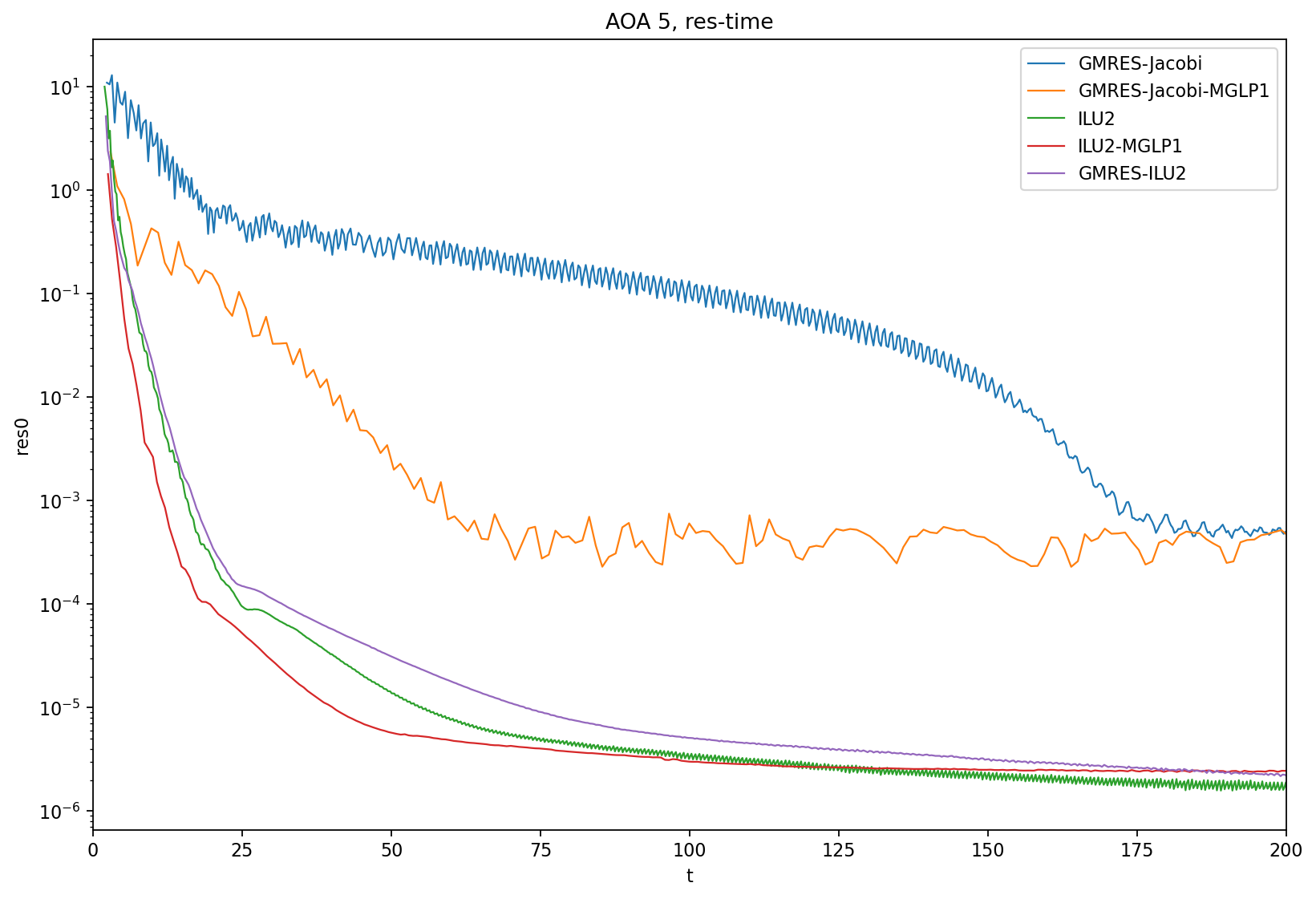
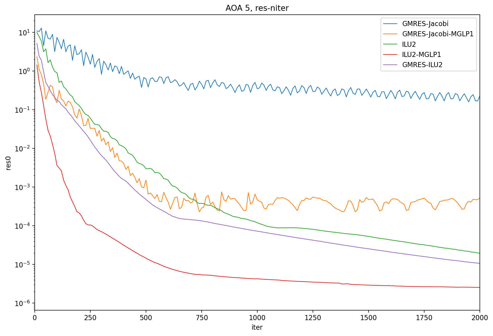
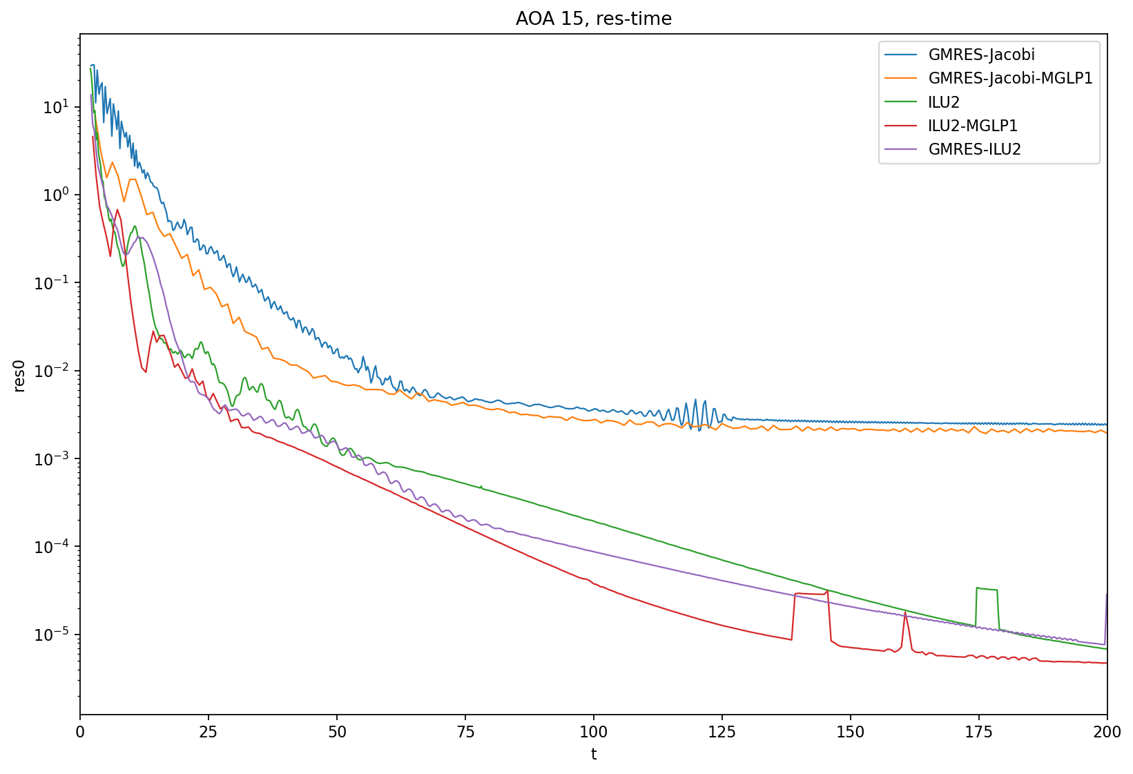
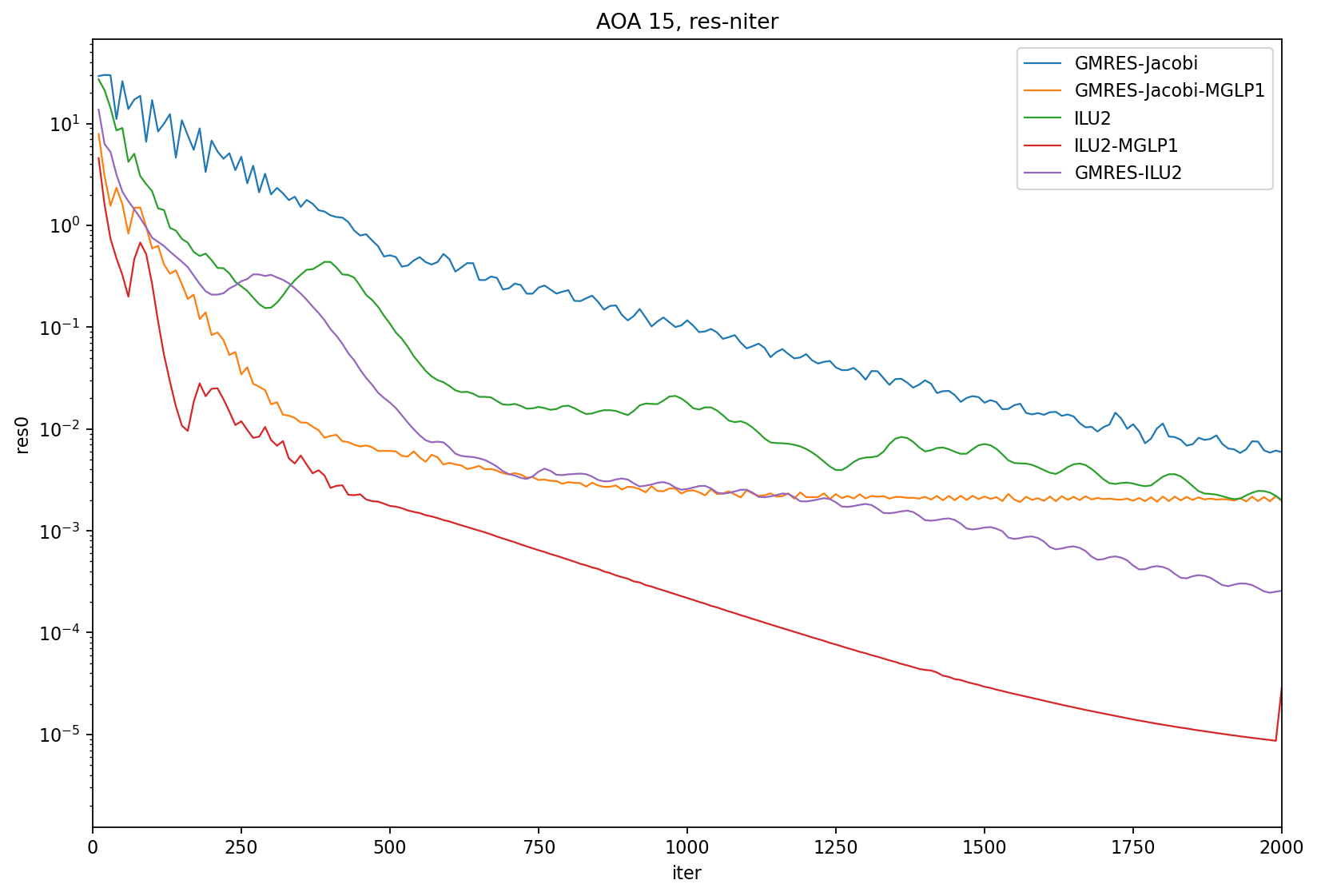
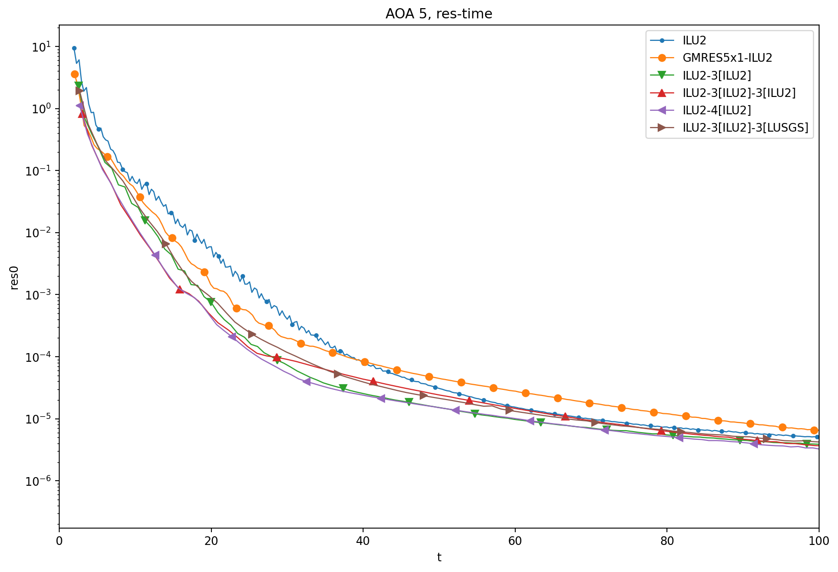
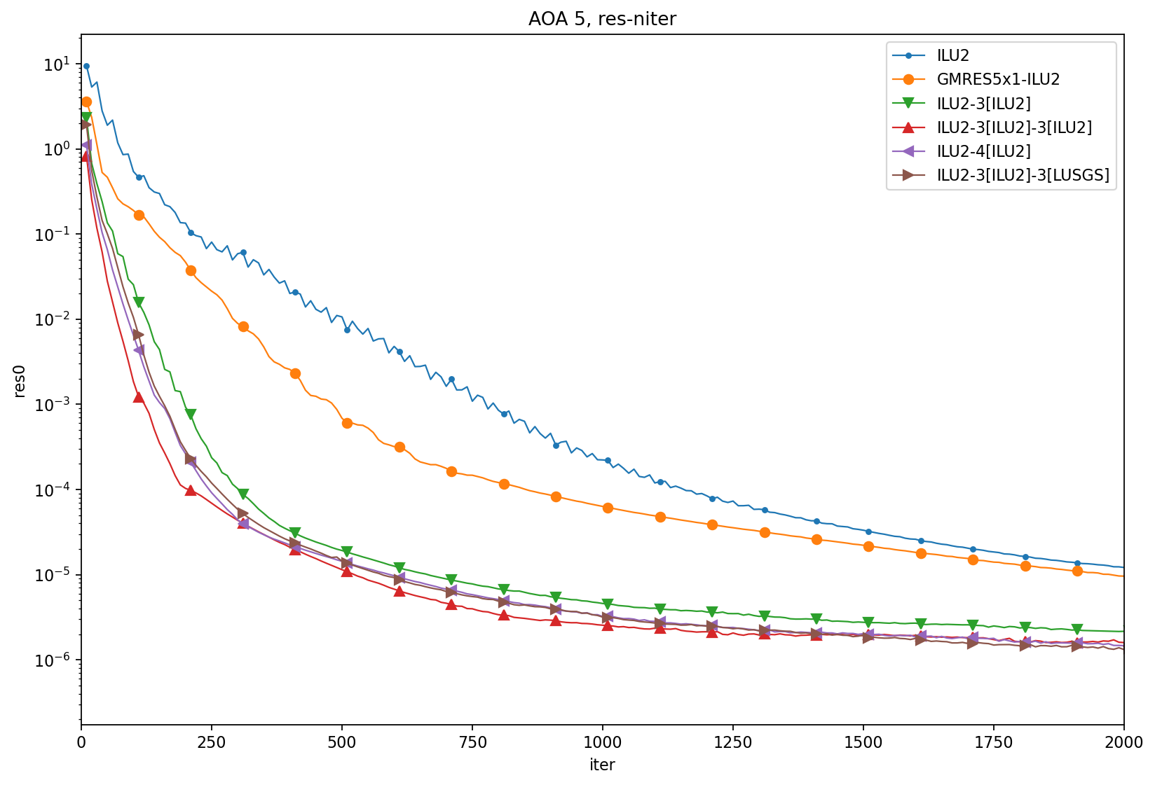
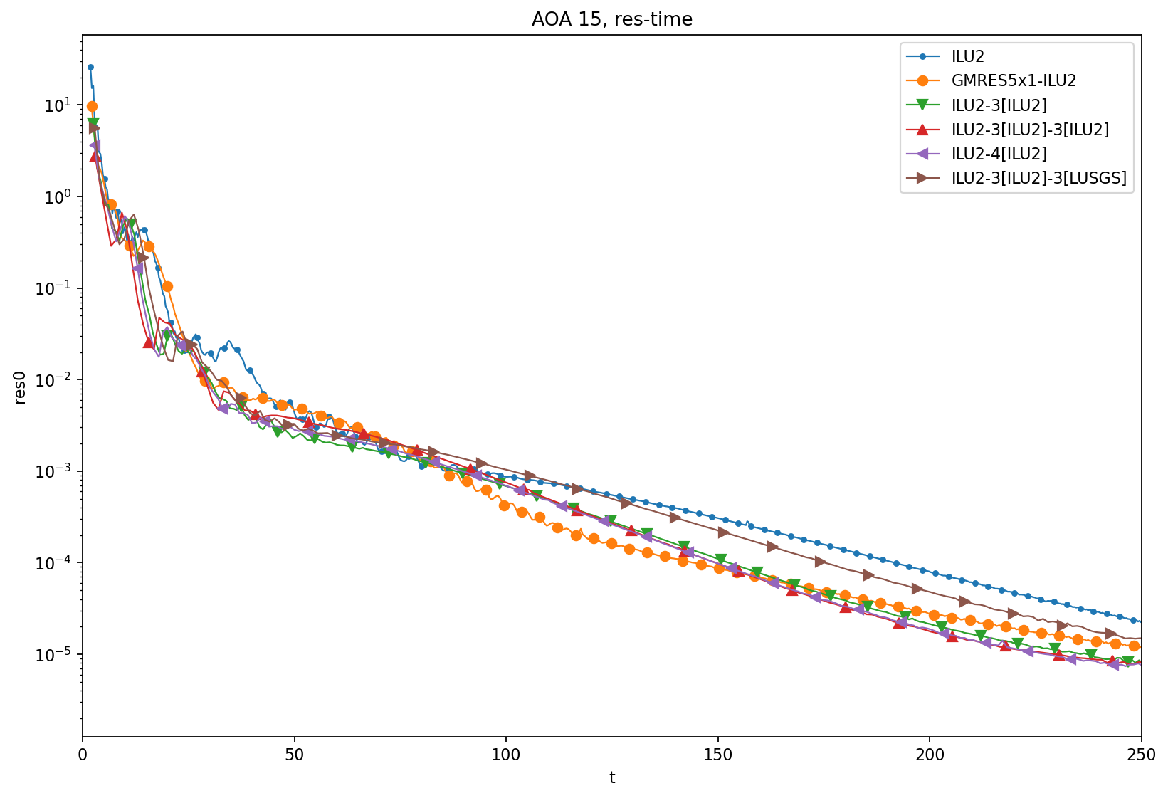
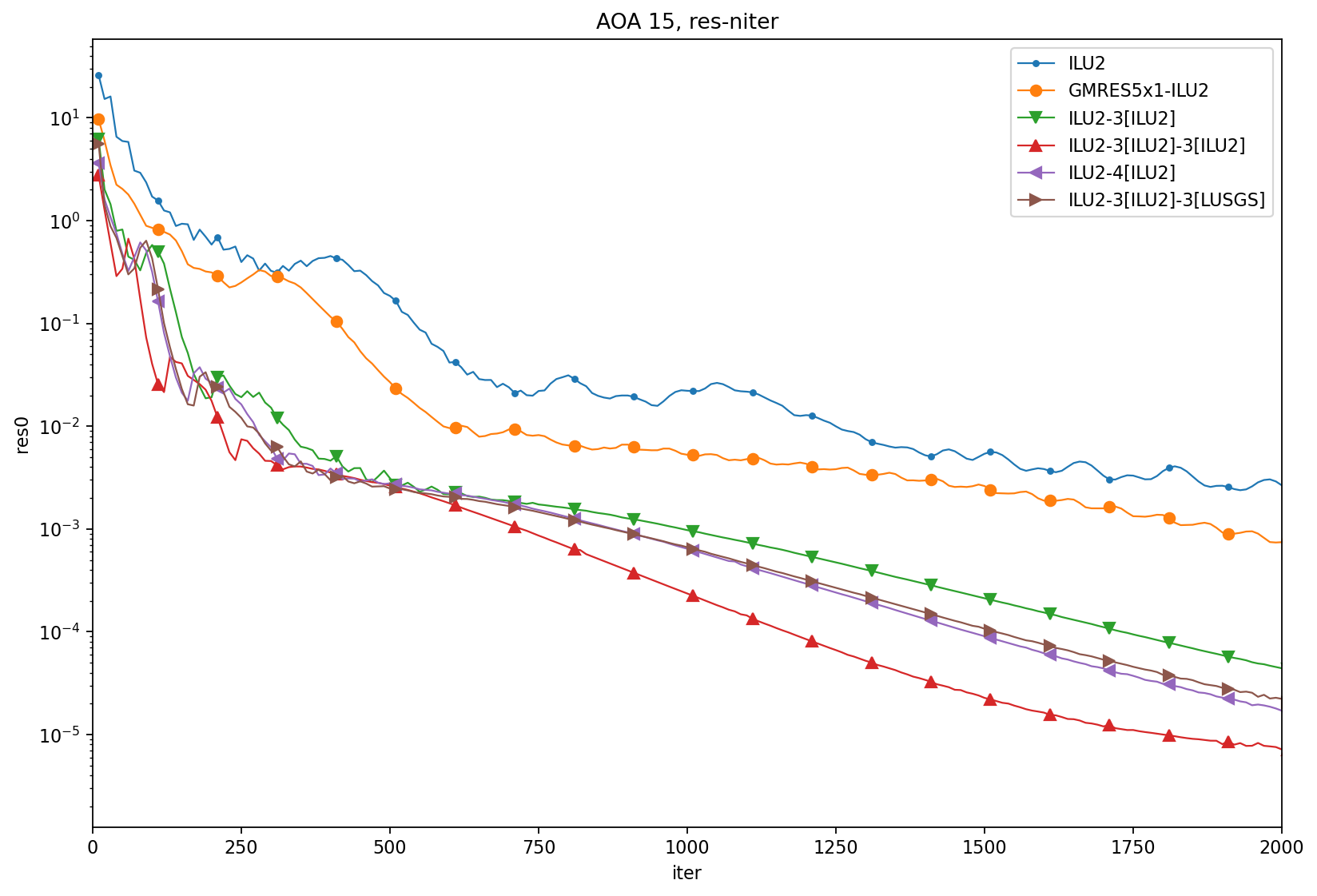
Test 1: 1 layer
NACA0012 foil, Re 2.88E6, Ma 0.15
GMRES k=5, restart=2
Jacobi or ILU-2
np=24
MGLP1:
- P1: ilu2 4 times
AOA = 5
AOA = 15
Test2: 2 layers
NACA0012 foil, Re 2.88E6, Ma 0.15
np=16
MGLP1:
- P1: ilu2 n1 times
- P2: ilu2 n2 times
AOA = 5
AOA = 15
Test 3: CRM CL=0.5
CRM no wing no plyon, AE @ AoA2.75
CL = 0.5, DPW6 settings
最终的阻力系数:
| |
算例 Brief
- 相对于无MG收敛加速:有时明显,有时比较微弱
- P=0的加入效果不明显,很难保证加速
- CRM:
- 加入MG对CL收敛没有加速
- 这应该和CL Driver有关
- 残差收敛似乎加速明显
- 需要针对此进行测试
- 加入MG对CL收敛没有加速
Test 2+: NACA 0012 AOA 15
With LLF flux on MG operator
With ignore vis on MG operator
With Implicit Residual Smoothing
IRS: Implicit Residual Smoothing
Using central form (fastest) (good for low mach) due to Jameson.
$$ \tilde{u}_i + \varepsilon \sum_{j\in S_i}{(\tilde{u}_i - \tilde{u}_j)} = u_i $$When $\varepsilon\rightarrow 0$, no smoothing.
Results:
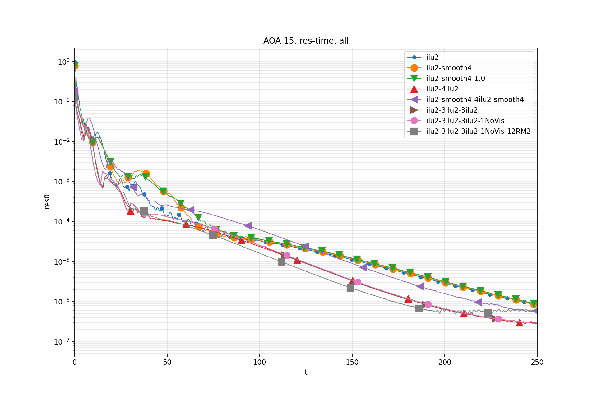
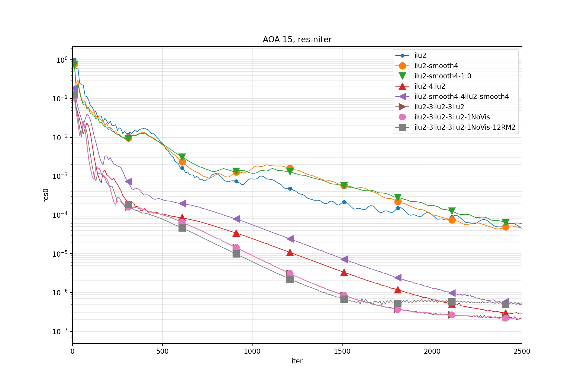
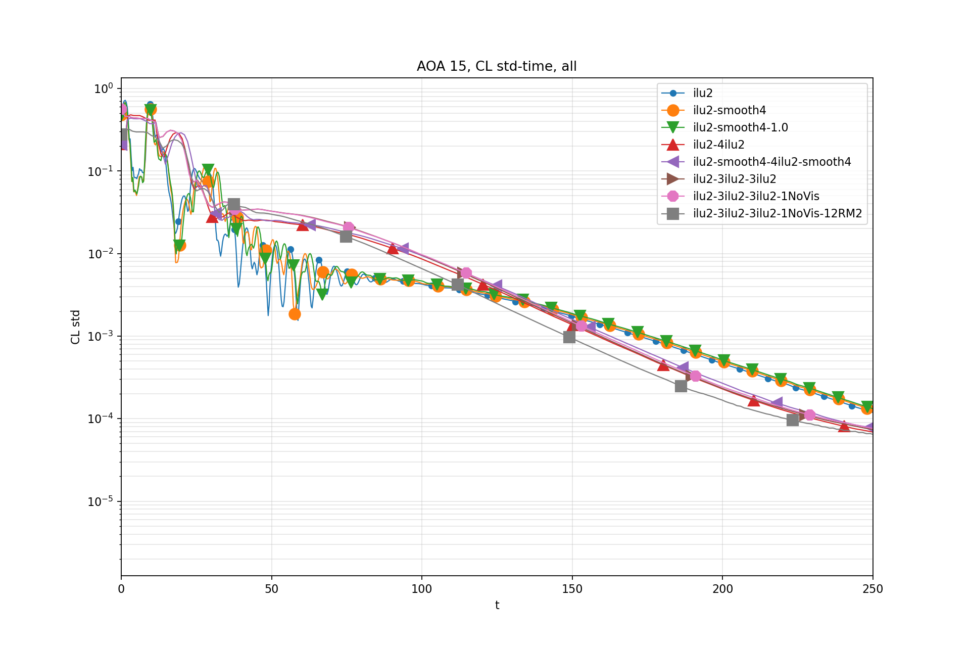
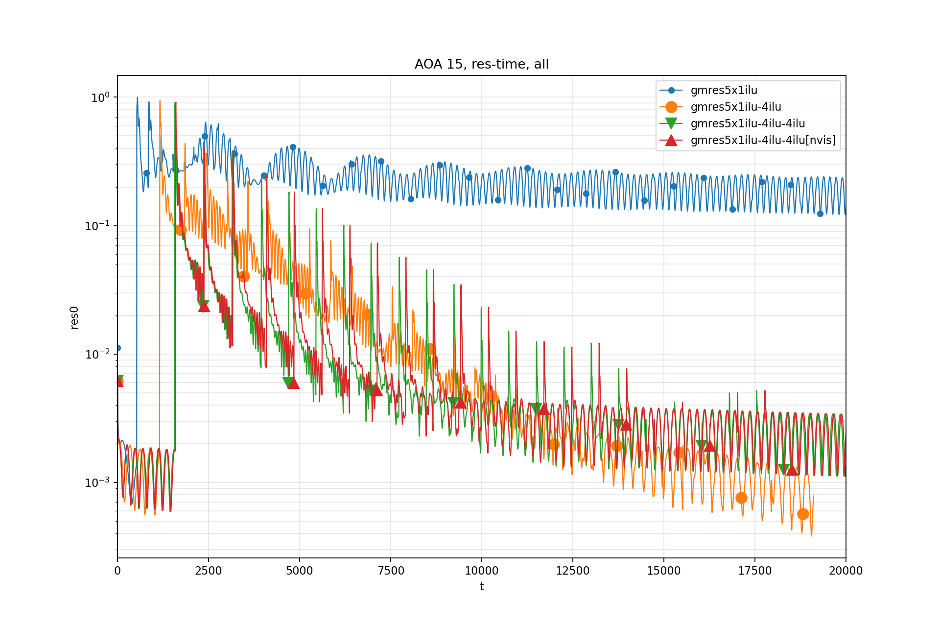
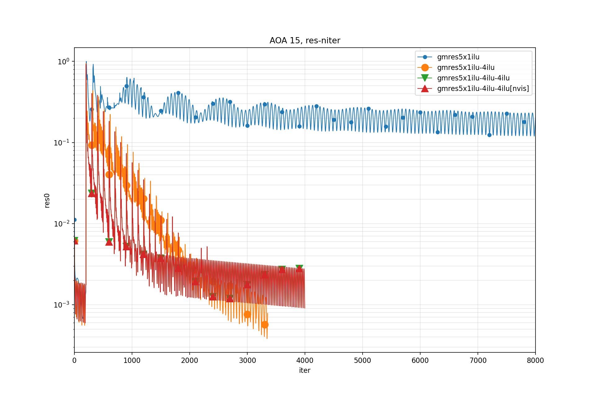
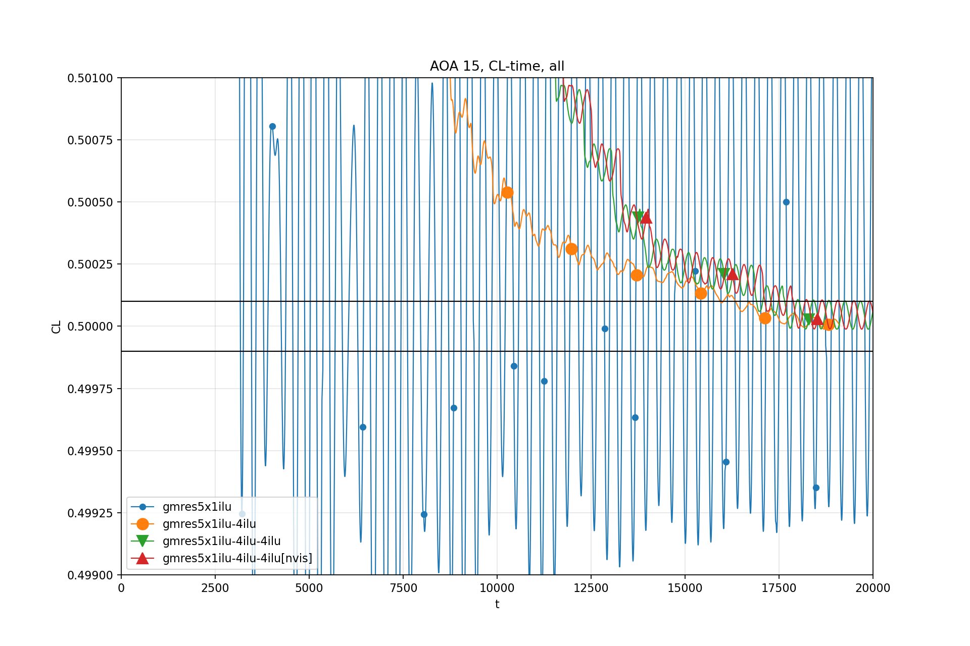
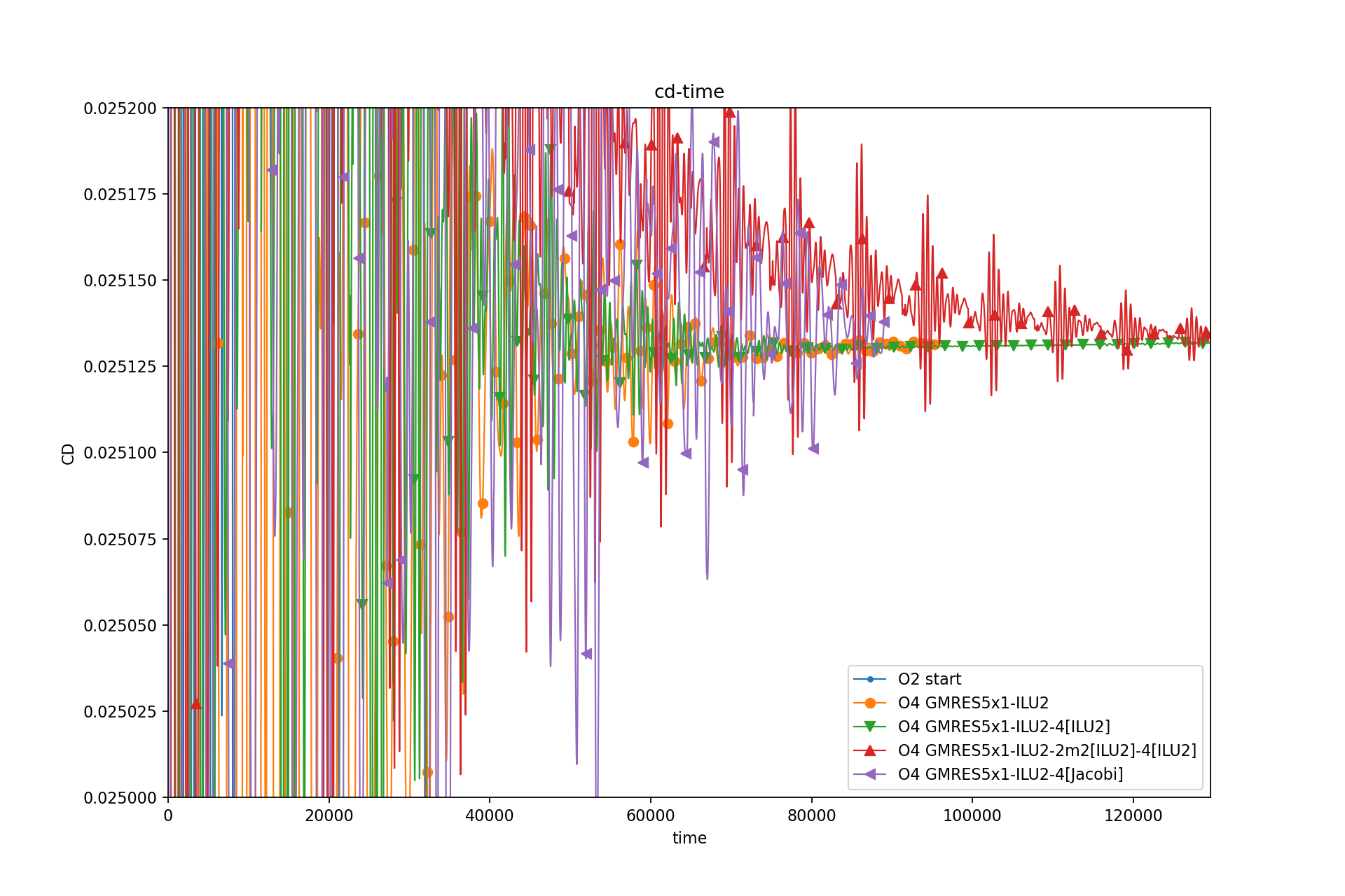
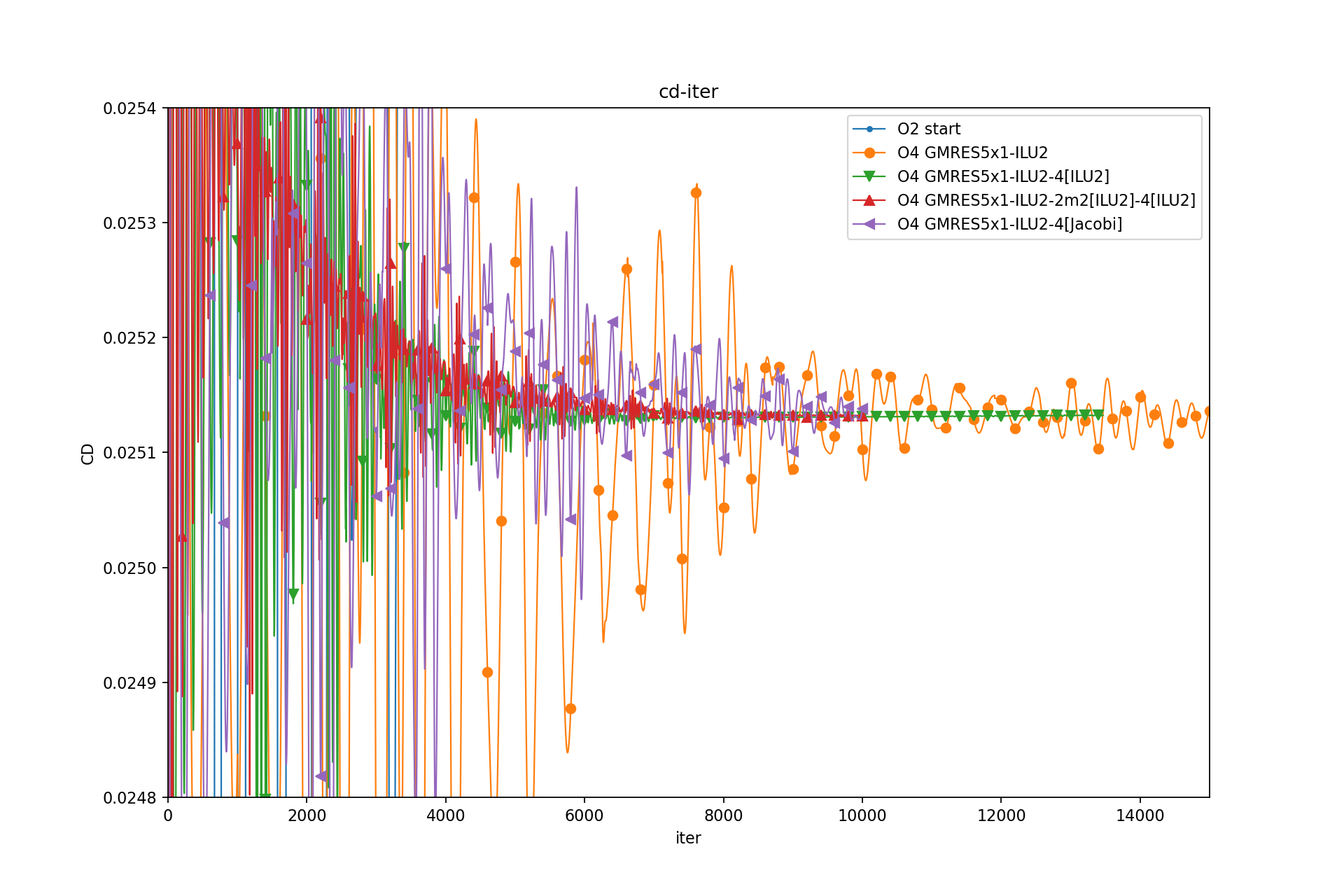
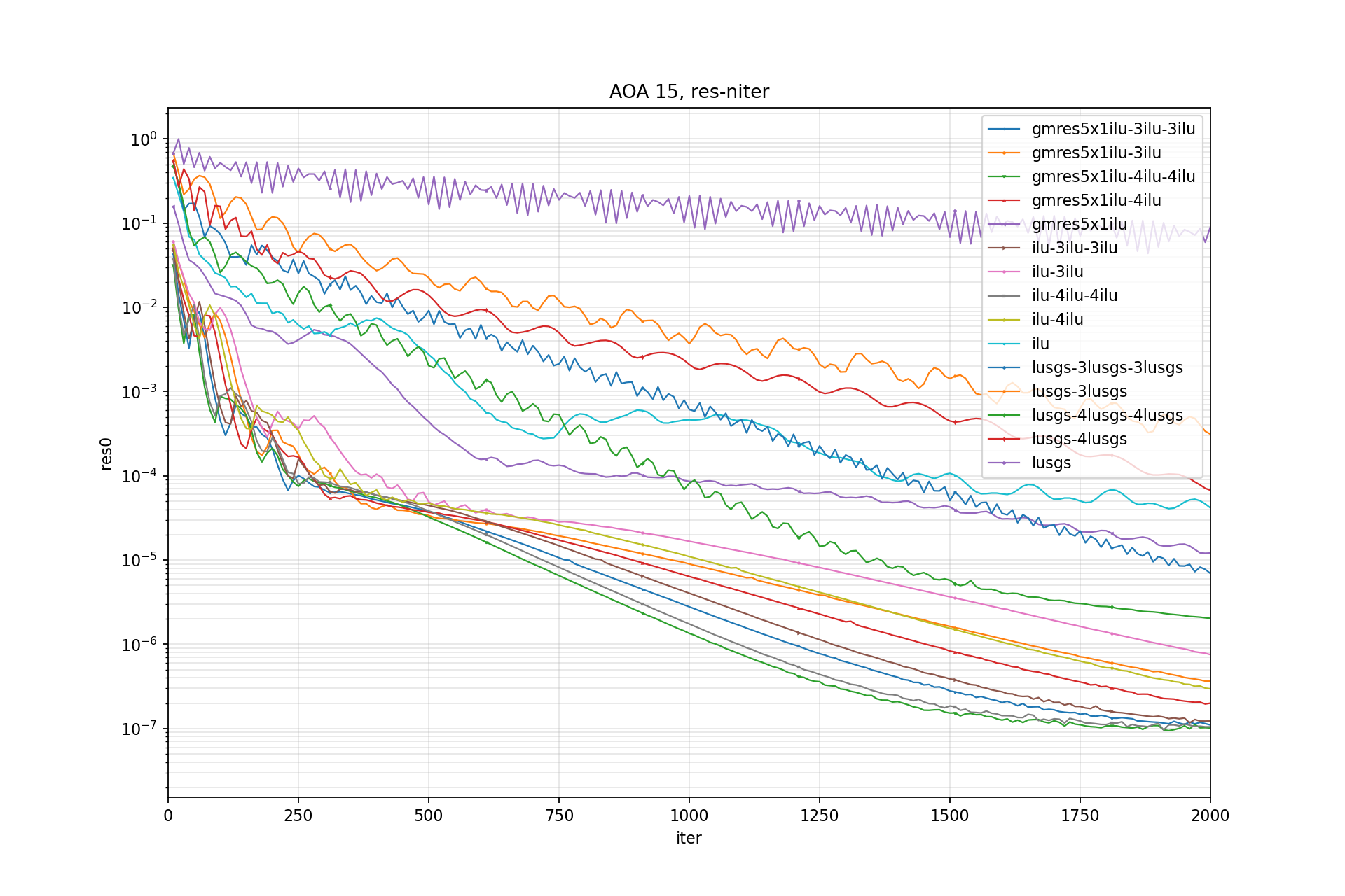
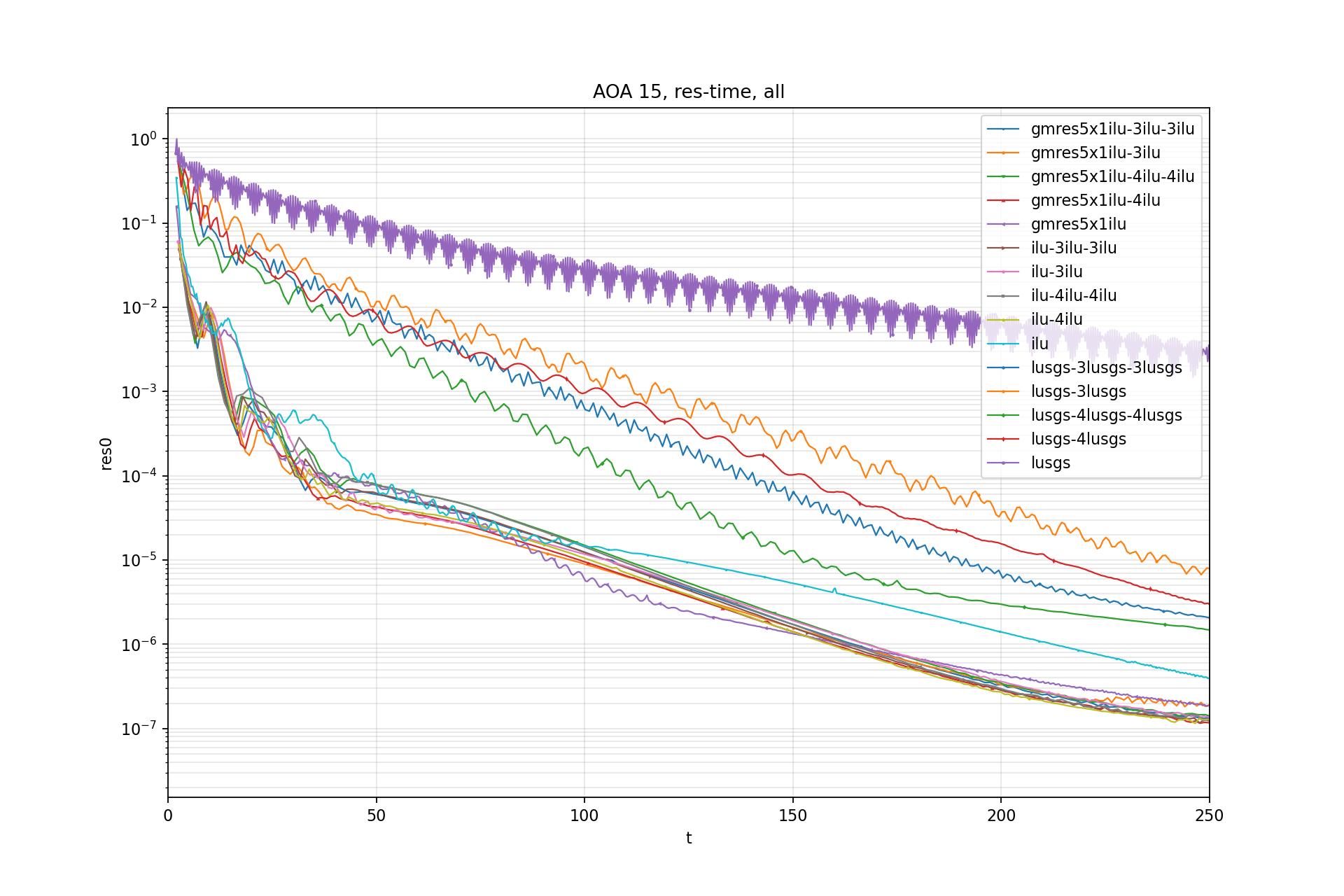
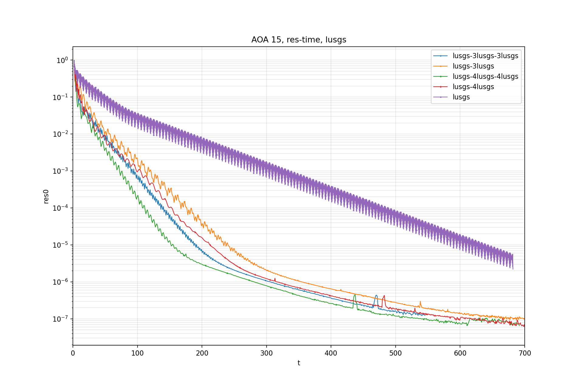
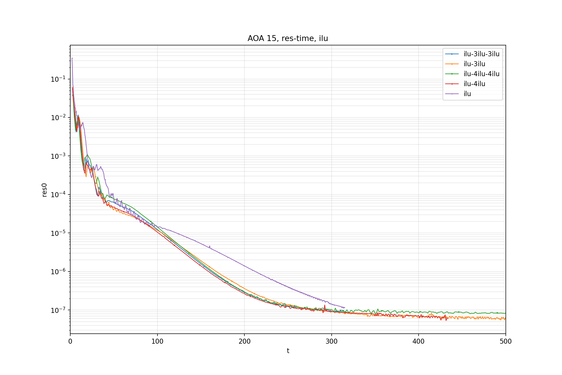
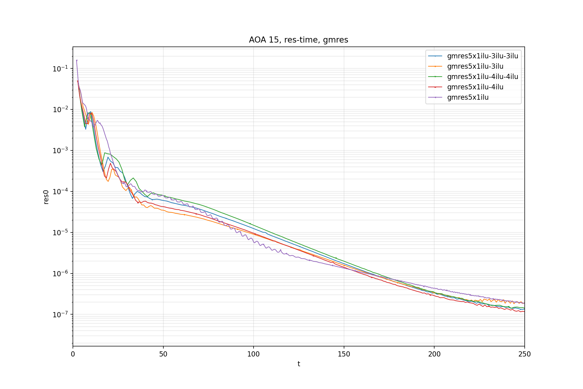
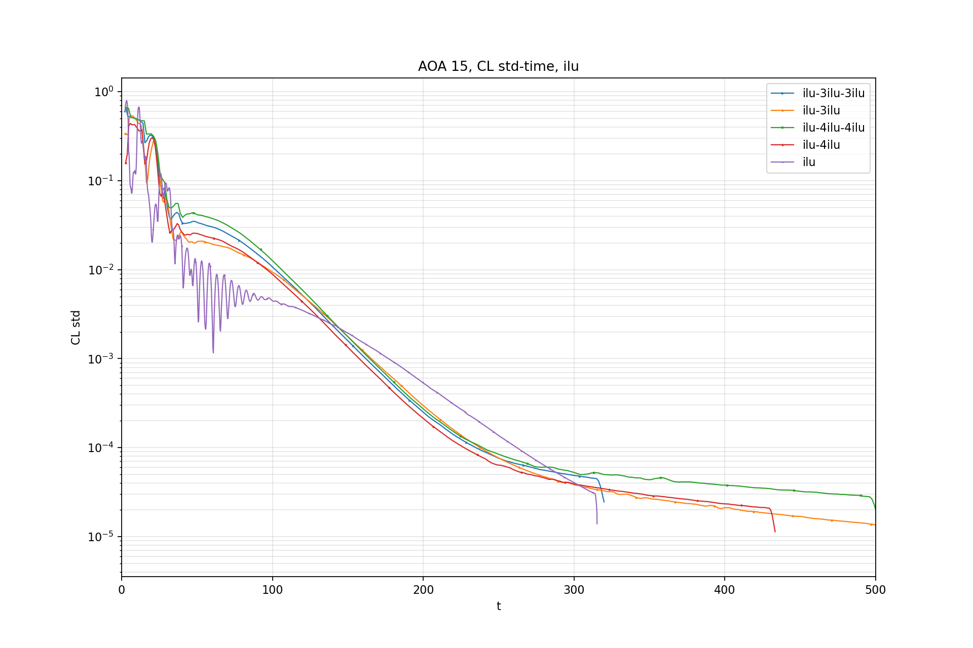
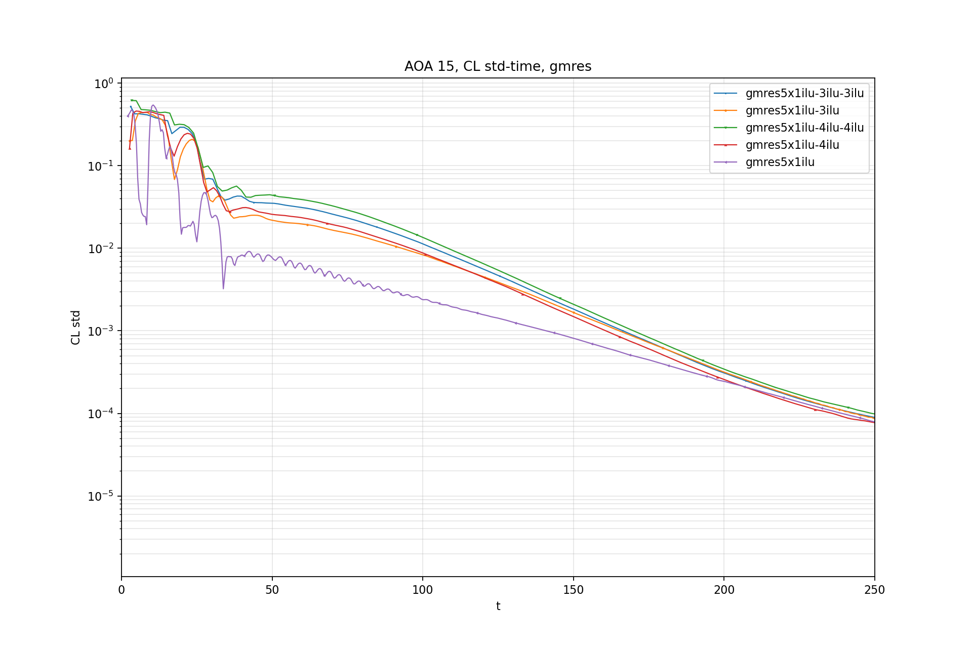
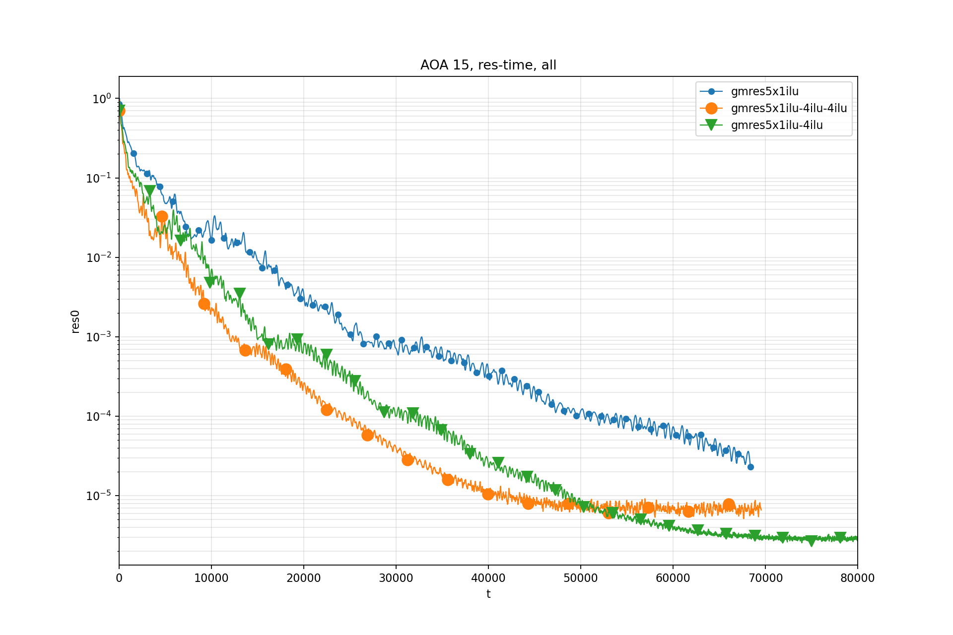
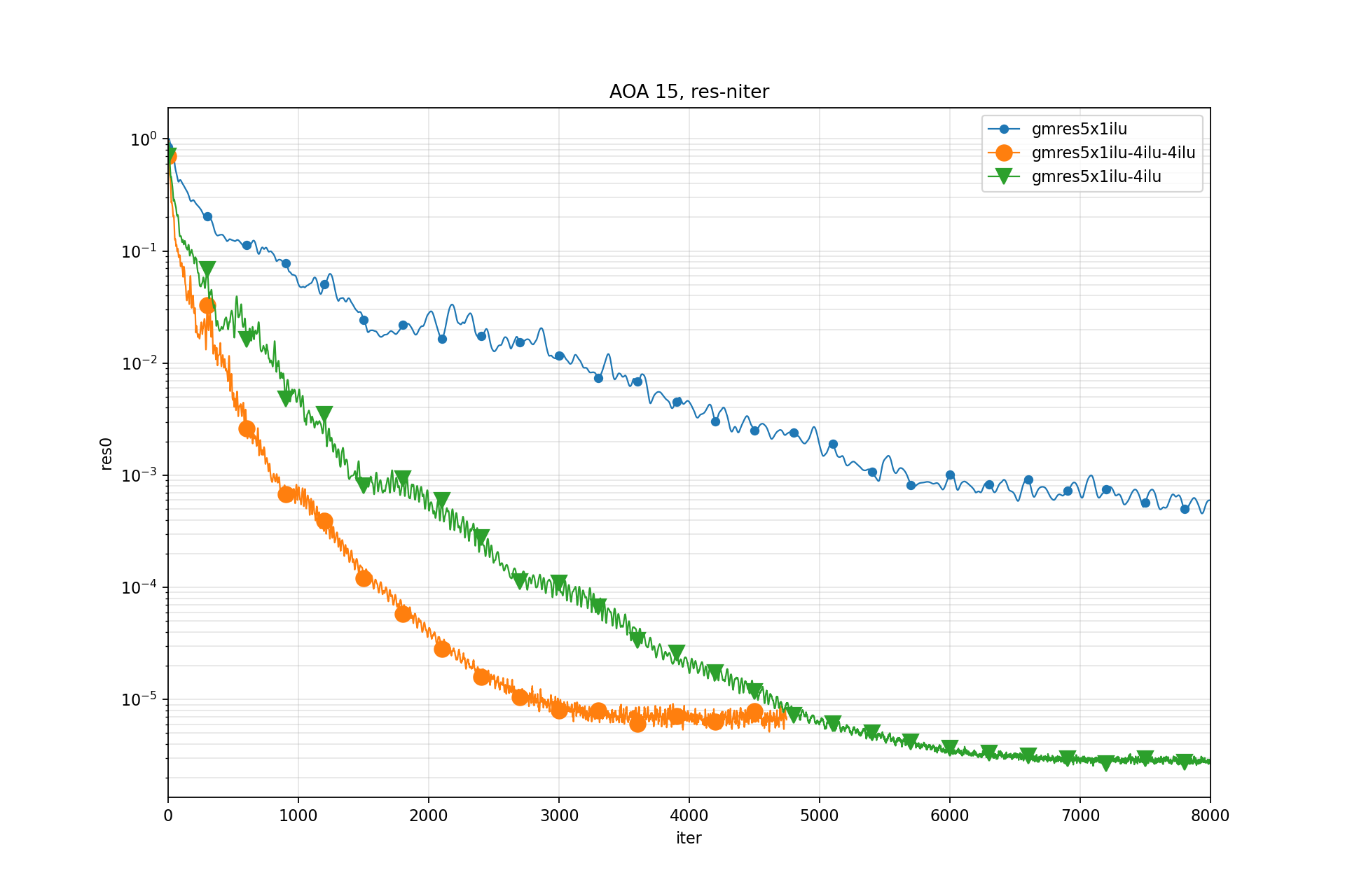
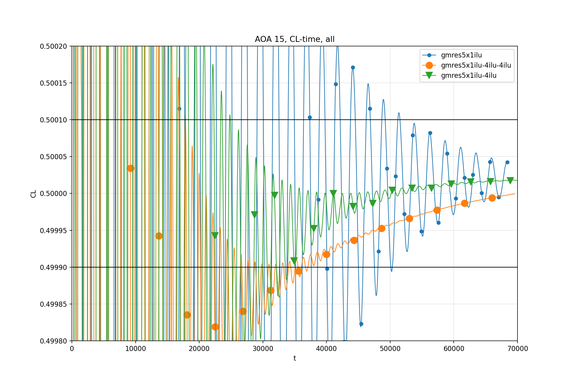
Test 4: NACA 0012 AOA 15
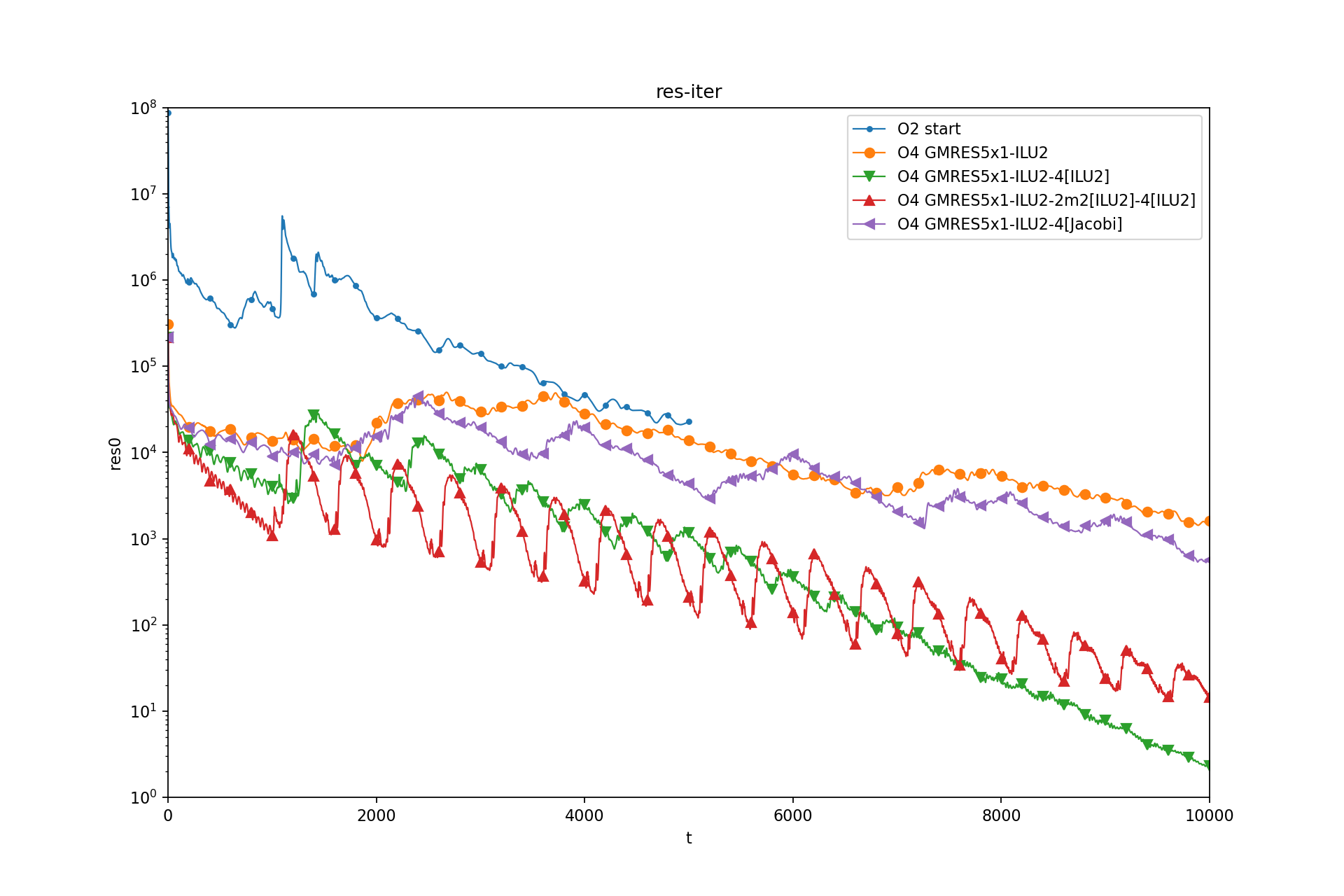
Residual redefinition
此前绘制的都是element-wise L1 残差
$$ \|\mathbf{r}\|_{e} = \sum_{i}{|r_i|} $$此后改用volume-wise残差:
$$ \|\mathbf{r}\|_{v } = \sum_{i}|r_i| \overline{\Omega}_i $$Residual-Iter:
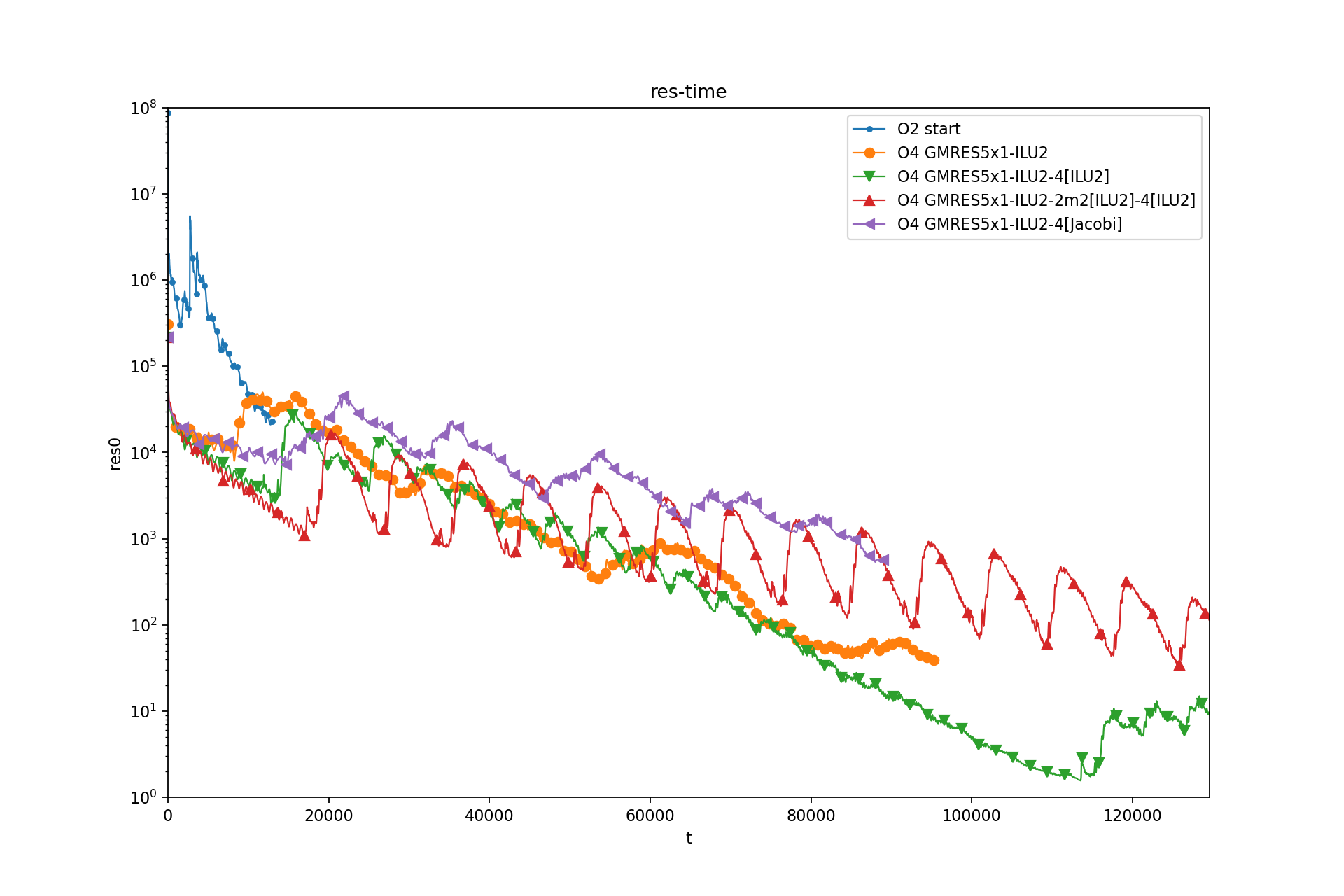
Residual-Time:
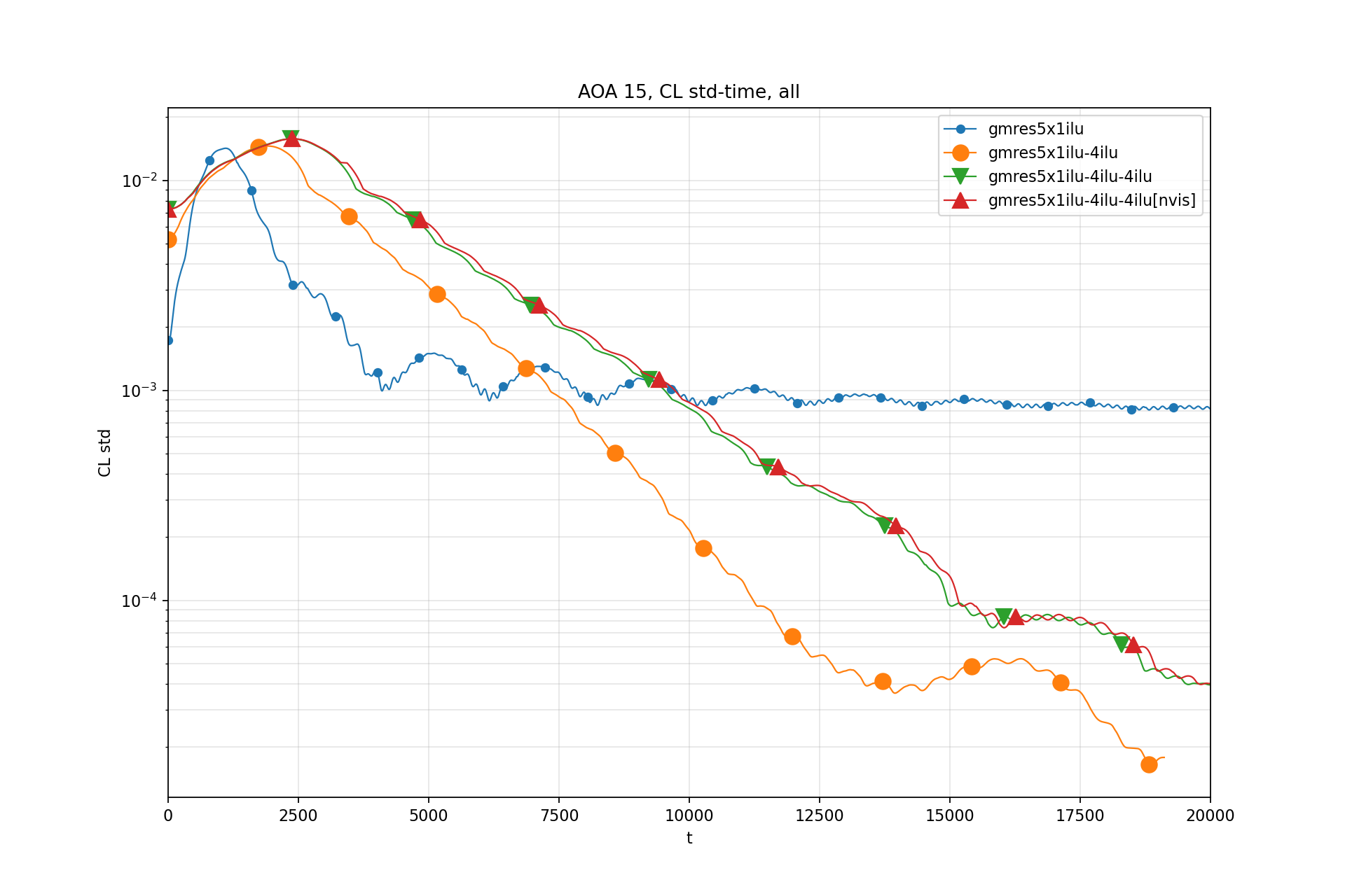
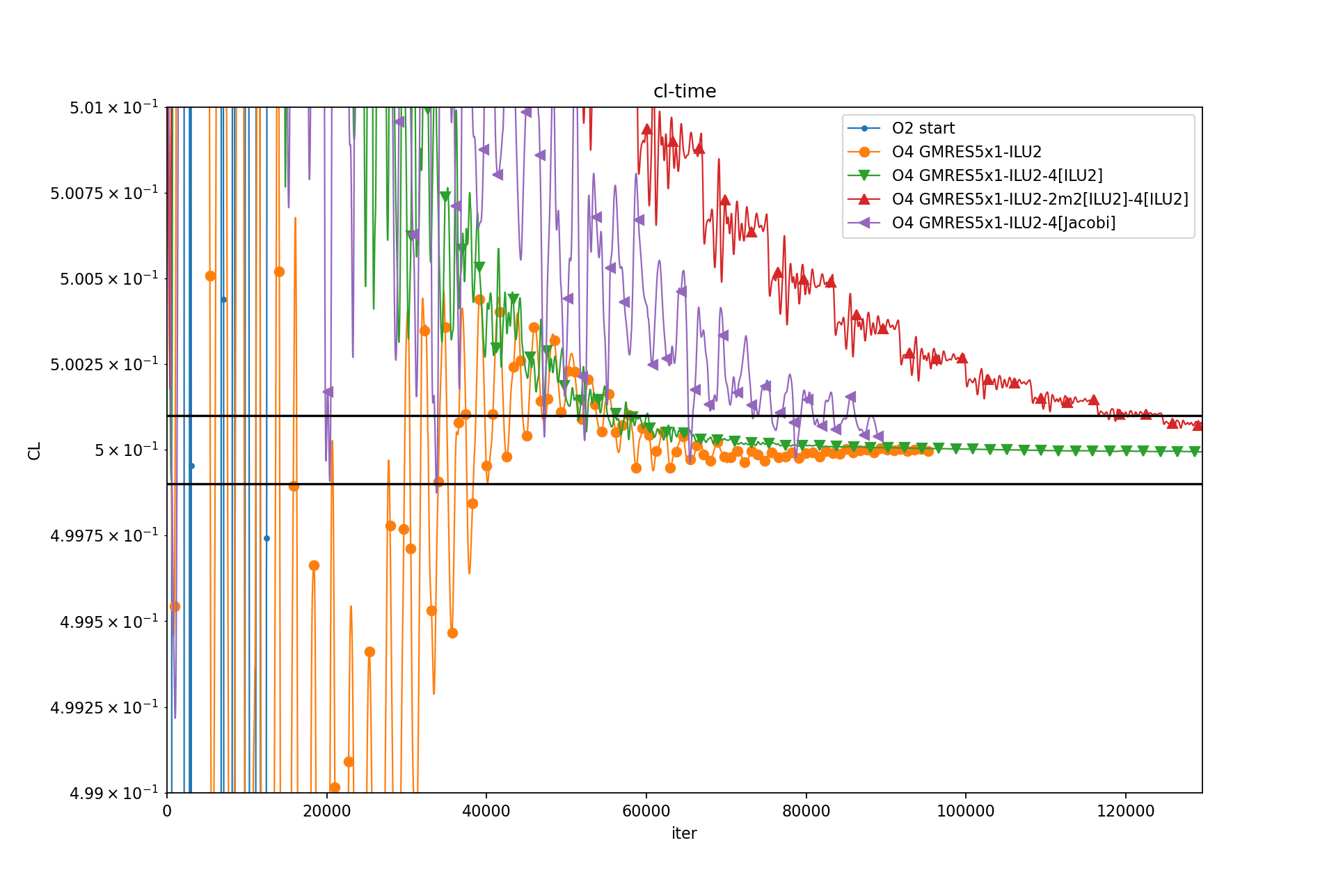
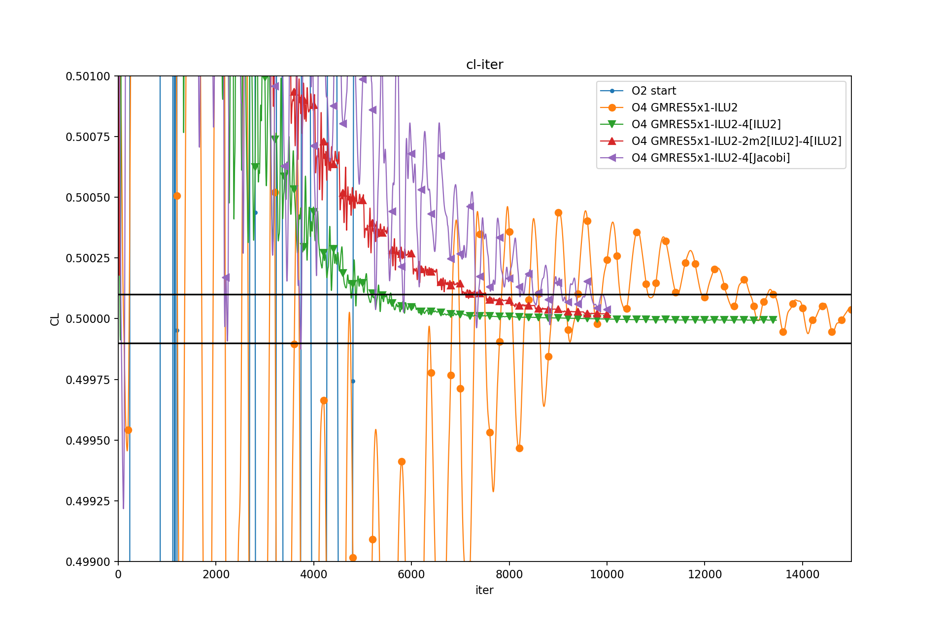
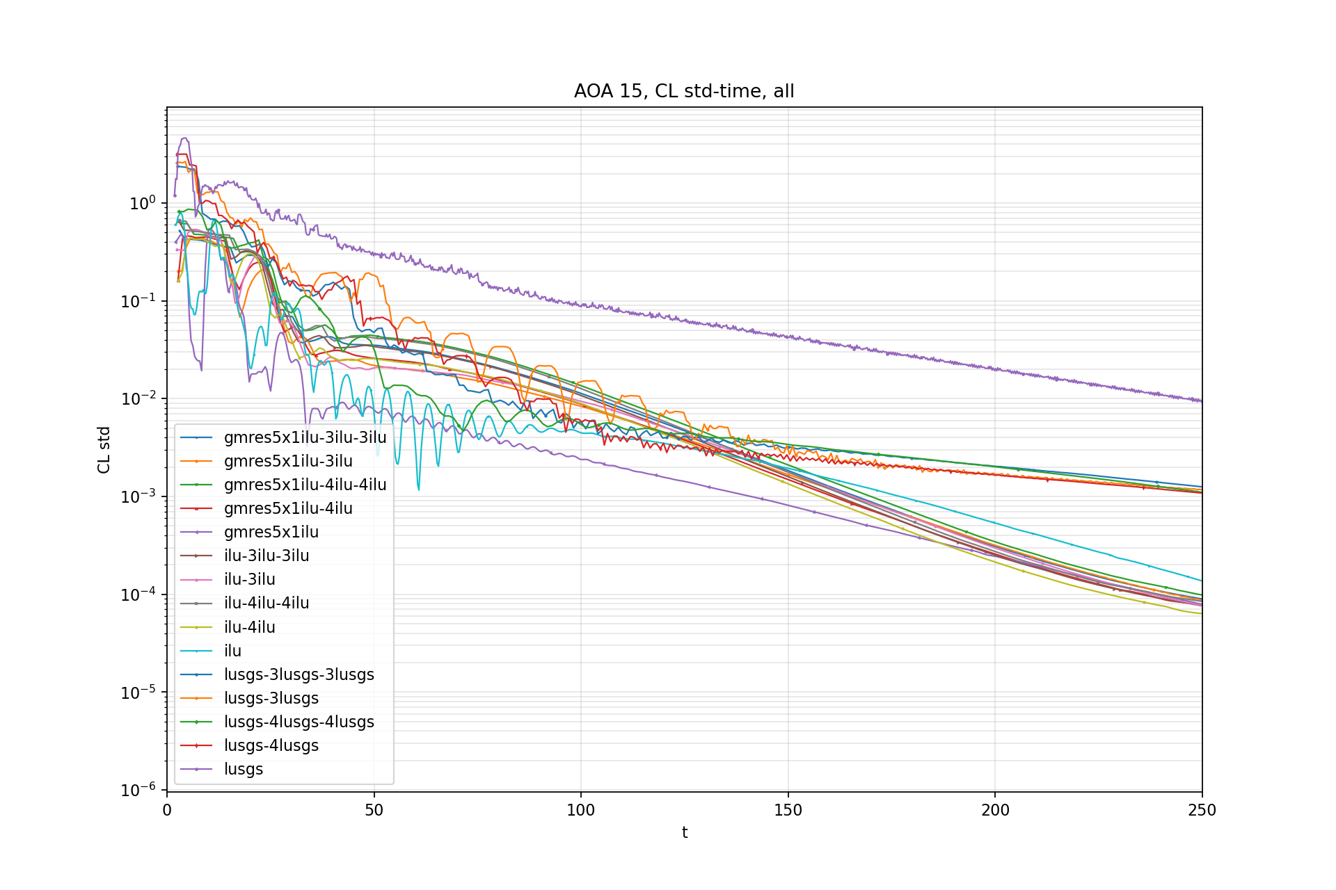
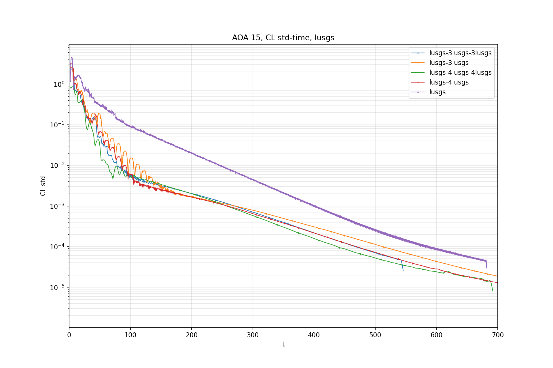
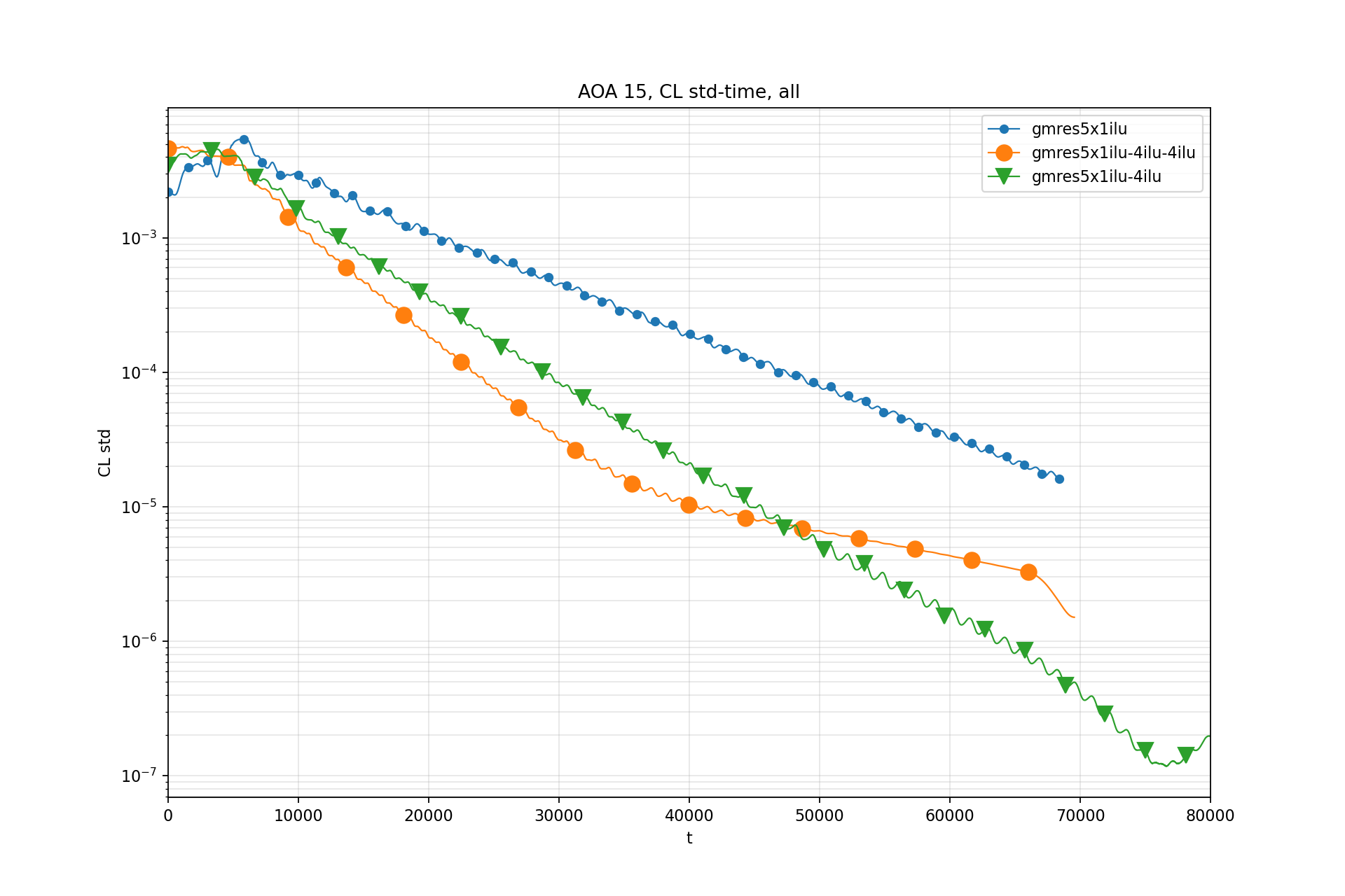
CL std - Time:
CL std is windowed standard deviation of CL.
Window size: 100 iterations (now downsampled by 10)
Test 5: CRM CL ~ 0.5
CRM no wing no plyon, AE @ AoA2.75
CARDC grid (2.6M)
Fixed AoA
Results:
Test 6: CRM Boeing F grid CL 0.5
CRM no wing no plyon, AE @ AoA2.75
With CLDriver